Category: Research Blog

Tap a thin panel, such as an aircraft skin, and it rings at a set of well-defined frequencies. Each frequency belongs to a mode shape, a pattern of deflection the panel likes to vibrate in, and for small vibrations these modes are wonderfully well behaved. They are decoupled from one another, and any motion can be written as a sum of them.

Tap the panel harder and this stops being true. Once the deflection grows to something like the panel’s own thickness, bending it also requires stretching, and stretching a membrane is a far stiffer proposition than bending it. The panel’s stiffness is now dependent on the amount of deformation, which means that frequencies of vibration change with amplitude, modes begin to trade energy, and the tidy catalogue of independent mode shapes falls apart. One of the challenges is that engineers increasingly want to operate in this regime but predicting what happens is expensive. A finite element model of a real component may carry a million degrees of freedom, and charting its nonlinear dynamic behaviour can take weeks of computer time.

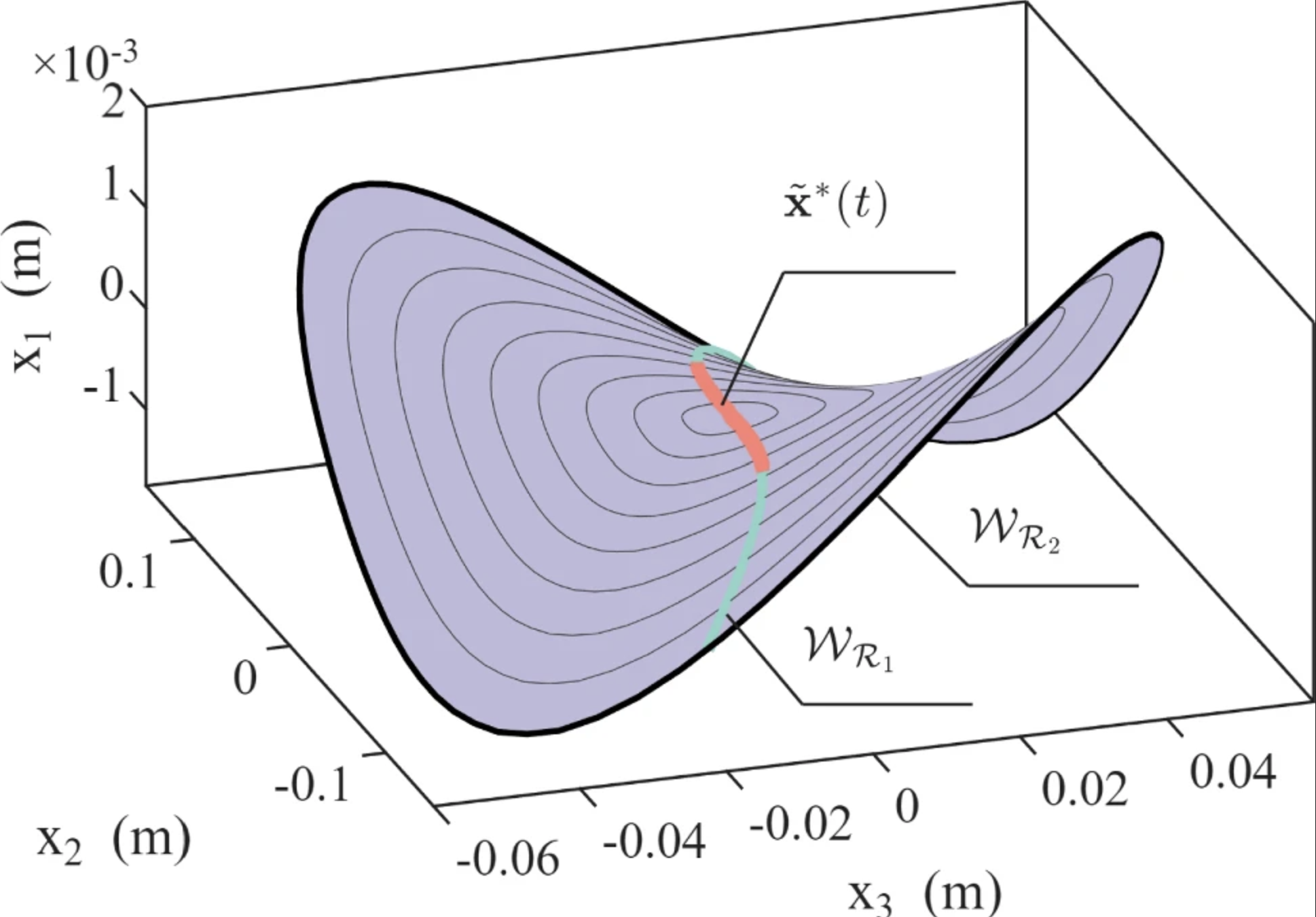
The standard escape route is a reduced-order model, or ROM. The insight behind this approach is that although the model may have a million degrees of freedom, the motion you actually care about does not weigh all degrees of freedom equally. Instead the motion is confined to a thin, curved surface threading through the million-dimensional space of possible deformed shapes. If you can find that surface, and describe it with two or three coordinates, then you can discard the rest and a simulation that took weeks now takes minutes.

There is a catch though. Commercial finite element packages do not hand you the nonlinear equations of motion but are a black box: you supply loads and the solver returns displacements. So-called indirect reduced-order methods have to find the surface using only what a black box can give you. One of the oldest of reduced-order methods is based on a simple premise: push the structure with static loads shaped like the mode shapes you intend to keep, record how the structure deforms and where it ends up, and then fit a polynomial through the force–displacement response. The set of shapes reachable this way is what we now call the stress manifold, and the ROM amounts to declaring that the only shapes the structure can ever adopt are the ones lying on that surface.

Applied force methods have a reputation for working well and for being held together with rules of thumb. Our two companion papers (1, 2) in Nonlinear Dynamics, written with PhD student Max de Bono and Tom Hill, try to replace the rules of thumb with something an engineer can actually check. They split the problem of trusting a ROM into two questions that the literature has long run together.

Have I drawn the surface accurately?

That is the subject of the first paper, which is all about verification. Many previously assumed that the reduced equations are cubic polynomials, on the reasonable-sounding grounds that the full equations are cubic. However, when you condense a cubic system down onto a lower-dimensional surface, what comes out is not necessarily cubic. The true functions are smooth, so a polynomial will approximate them locally, but “cubic” is a local approximation in exactly the same sense that “linear” is.

Once you appreciate this, verification becomes a well-posed question: raise the polynomial degree until the description of the surface stops changing. We set out an automated algorithm for doing this that adds load cases where they are needed and otherwise touches the finite element model as little as possible, since every call to it is the expensive part.

As a demonstration, a curved double arch with over a million degrees of freedom was reduced to a two-mode ROM and verified in sixty minutes on a desktop computer, reproducing an internal resonance present in the full-order system.

Is it the right surface?

This is validation, the subject of the second paper, and it is much harder. A ROM can be a beautifully accurate map of the wrong territory. The classic failure is internal resonance: as amplitude grows and frequencies drift, two modes can wander into a simple whole-number ratio, lock together and start trading energy back and forth. If the second mode is not among the ones you kept, your ROM has no ability to represent it and will report a periodic vibration that does not exist in the real structure.

The usual remedy is to check against full-order simulations, which defeats the point of building a ROM in the first place, or to build a larger ROM and see whether the answer moves, which is expensive and requires guessing which modes to add.

Our approach starts from a simple observation: to find out whether an orbit would survive in a larger ROM, you do not need the larger ROM. You only need its slope at the points you have already visited. Take a vibration predicted by the small ROM, and at every instant during the cycle attach the flat tangent plane of the bigger surface. Stitched together over one period, these planes form a time-varying validation manifold, and the question becomes whether the orbit, now permitted to drift, actually does so. That question turns out to be a set of linear differential equations with periodic coefficients, which is cheap to solve. If the sideways displacement stays at zero, the orbit exists in the larger ROM and the smaller set of modes was sufficient. If it does not, the solution names the modes you need to add. The stability of the same equations flags bifurcations the small ROM has missed.

The gradients this requires can be extracted while the original surface is being built, so the extra cost is modest. In the double arch again problem, a two-mode ROM of a 100,000 degree-of-freedom model, exhibiting internal resonance, was built and fully validated in under fifteen minutes. Refining the mesh to a million degrees of freedom pushed this to 170 minutes. The equivalent check by full-order simulation would take days. Crucially, nothing in the procedure assumes that an internal resonance exists, or which modes might be involved.

This “validation backbone” is a diagnostic tool and not a prediction. The further an orbit drifts off the original surface, the less the linearisation that was used to construct it can be trusted. Therefore, it tells you reliably that a result is wrong but it does not replace building the larger ROM to find out what is right.

Stepping back, the interesting question here is not really which reduction method is most elegant. Methods built on invariant manifolds are more rigorous and, dimension for dimension, more efficient. But dimensional efficiency is not the same as computational efficiency: a point on a stress manifold is cheap to find and comes with no awkward questions about existence or uniqueness, so a slightly larger reduced model can still be quicker to build and interrogate than a smaller, more sophisticated one. What has really restricted applied force methods in the past is not their mathematics but the absence of any principled way of knowing when you can trust what it produces.

Both papers are open access, and every result in them can be reproduced with AFR Tool written by Max de Bono.

Think of a structure’s elastic behaviour as a ball resting on a hilly landscape. Every dip in that landscape is a shape the structure is happy to hold on its own, and every ridge between two dips is the energy barrier that keeps it there. A bistable structure, such as a hair clip or a shallow arch pushed inside out, is a ball sitting in one of two valleys. To change its shape, you push the ball over the ridge and let it fall into the neighbouring valley.

But there is a second way. Instead of pushing the ball over the ridge, you can reshape the hillside underneath it until the valley it is sitting in ceases to exist. The ball has nowhere to go but downhill.

This distinction matters because the usual routes to shape-changing, morphing structures have drawbacks. Materials that expand, contract or bend in response to heat or moisture tie the speed of shape change to the intrinsic speed of the material, such as thermal diffusion. Shape changes can take minutes or hours, and holding the new shape often means keeping the stimulus switched on. Multistable structures fix the latter energy problem, since both shapes are self-equilibrated, but something still has to supply the push across the energy barrier to initiate shape change, and doing this reliably in a larger-scale structure is not easy.

Our recently published paper in the International Journal of Solids and Structures asks a different question:

Where should active material be placed inside a structure so that heating or cooling destroys one of its stable states?

We call this strategy active stiffness tailoring. As a proof of concept, we demonstrated this strategy on a shallow arch 3D printed from two commercial photopolymers. The two polymers respond very differently to temperature, such that over the tested working range of 30 °C to 60 °C, the ratio of their stiffnesses reduces from roughly 355:1 to roughly 14:1—a 25-fold change. Crucially, it is this change in ratio that drives the mechanics, and not the absolute stiffness of the components. Scaling both materials by the same factor rescales the energy landscape but leaves its shape, and therefore the stability of the arch remains untouched. But if the ratio is changed, the strain energy redistributes between the stiff and compliant regions, changing the energy landscape itself.

This gives us a design variable to optimise: the boundary between the two materials through the thickness of the arch. We optimised this interface to optimise the relative proportion of the two material through the thickness in order to maximise the strain energy released at the point where the arch loses stability and transitions into the second state. A larger energy release means a more decisive snap and a design less likely to be derailed by manufacturing scatter.

Two designs were optimised, and they behave in opposite thermal directions. One is bistable when hot and becomes monostable on cooling (snaps upon cooling), and the other is bistable when cold and becomes monostable on heating (snaps when heated). The material layouts that achieve this are not ones you would have guessed by eye: the optimiser places active material where its softening with temperature most severely degrades the bending stiffness that sustains the everted shape, and keeps passive material where it is needed to preserve bistability before actuation.

We then tested the snap-upon-heating design in a water bath to test and demonstrate the phenomenon experimentally. While the shape transition occurred as expected, the measured transition temperature exceeded our predicted temperature by nearly 11 °C. Frame recoil, uncertainty in the material data and thermal expansion are all possible explanations for this discrepancy.

The result we find most interesting is about timescales. Heating the water bath took minutes. The snap itself took less than a second. Once the critical stiffness ratio of the two materials is crossed, the rate of shape change is independent of how fast the polymer responds itself and rather is set by how much elastic energy is released into motion. The stimulus and the response have been decoupled, which is exactly what conventional shape-memory actuation cannot offer.

More broadly, this is another example of instabilities being used for design rather than being avoided as a failure mode. In this case, elastic nonlinearity does the job that sensors, actuators and control systems often do together. Where the structure is stable, how much energy it will release and where it ends up can all be programmed into the material layout at the printer, and then triggered later by an ambient temperature change. No motors, no wiring, no control loop. There is also no reason to assume that the stimulus has to be heat — light, moisture, electric and magnetic fields would all serve as potential ambient actuation sources, provided they change stiffness enough to reshape the energy landscape.

Wind energy is expected to be one of the central pillars of a low-carbon electricity system, and for the past few decades the industry has pursued a single, simple strategy to push costs down: build bigger. Each new turbine generation carries a larger rotor than the last, because — up to a point — a longer blade sweeps more area and captures more energy. But the trend cannot continue indefinitely. As blades grow, the mass of blades, generator and nacelle climb faster than the power they produce, and the practical headaches of manufacturing and transporting large components begin to factor. Eventually the cost of going bigger outweighs the extra energy, and the levelised cost of energy (LCoE) — the price of electricity averaged over the lifetime of the turbine — stops falling.

One way around this ceiling is to stop thinking of a turbine as a single rotor. A multi-rotor wind turbine (MRWT) replaces one very large rotor with a coplanar array of many smaller rotors mounted on a shared support structure. The installation occupies a similar footprint and produces the same total power, but the individual blades are short enough to be considerably easier and cheaper to build and transport. Smaller rotors also mean less material overall and the system can keep producing energy even if a rotor fails.

This is the promise, at least. The difficulty is that nobody can yet say with confidence how large these savings really are. The theoretical argument most often cited in support of multi-rotors — a “square-cube law” of scaling — is not borne out by simulation data, and there are few physical installations or detailed design studies to check against. Most existing studies take shortcuts: they reuse rotors designed for conventional single-rotor machines, simplify or ignore important ways the structure can fail, or tend to conclude that increasing rotor count indefinitely always lowers costs — a result that is unlikely to hold in practice.

In a recent paper presented at the Torque 2026 conference, we set out to close that gap with a more honest design process. The work uses an in-house aeroelastic optimisation tool, ATOM, to design a multi-rotor turbine from first principles. “Aeroelastic” simply means the calculation accounts for both the aerodynamic loads imposed by the wind and the way the structure deforms in response; “optimisation” means the software automatically searches for the design that minimises cost. Importantly, the rotors are not borrowed from single-rotor turbines — they are drawn from an open library of rotors (blog post here) we optimised specifically for the multi-rotor context in earlier work.

Designing a multi-rotor turbine means answering two intertwined questions at once: how many rotors to use, and how to arrange and size the support structure that holds them. We tackle this with a “tiered” approach. For each candidate number of rotors, the software lays out the arrangements that are geometrically feasible — square grids, hexagons, pyramid-like stacks — and then designs the lightest support structure that can sustain loads in each case, checking every member against strength, buckling and fatigue failure. The competing arrangements are ranked by cost of energy to choose the best one for that rotor count. As a demonstration, optimising the support structure of a seven-rotor, 3 MW turbine reduced structural mass by nearly 70%.

The ultimate aim of this work is not to hand industry a ready-to-build blueprint, but to make a fair comparison possible. Because we now optimise both the rotors and the structure that carries them — rather than scaling up off-the-shelf parts — the eventual head-to-head comparison against an equivalent single-rotor turbine should be more representative than previous attempts. This conference paper is a deliberately preliminary step: it demonstrates the framework on individual cases, and the next stage is to sweep across a wide range of rotor numbers to locate the genuine sweet spot for a given power rating. Only then can we offer a credible answer to the question if multi-rotor turbines actually make wind energy cheaper.

Wind energy is expected to play a central role in the global transition to low-carbon electricity. Over the past decades, the dominant design for wind turbines has been the single large rotor mounted on a tall tower. However, as turbines continue to grow in size, engineers face increasing challenges related to transportation, manufacturing, structural loads, and cost.

One alternative concept that has attracted growing interest is the multi-rotor wind turbine (MRWT). Instead of one very large rotor, a multi-rotor turbine uses many smaller rotors mounted on the same structure to achieve the same overall power output. This approach could offer several potential advantages: smaller blades are easier to manufacture and transport, maintenance can be simplified, and the system may continue operating even if one rotor fails. In some cases, interactions between the rotors may even slightly increase the total power generated.

Despite this promise, research on multi-rotor systems has been limited by a practical issue: the lack of suitable reference rotor designs that researchers can use for modelling and comparison. Most existing wind-turbine reference models were created for single-rotor systems and are not well suited to studying arrays of smaller rotors.

To address this gap, we have developed an open-source library of optimised wind-turbine rotors, covering rated powers from 100 kW to 1 MW. These rotor designs were created using aeroelastic optimisation methods, which consider both aerodynamic performance and structural behaviour. The optimisation process enabled the design of blades that balance energy production, structural safety, and material use.

A key feature of the library is that the designs are fully open and compatible with widely used simulation tools. This means researchers around the world can use the models directly in their own studies. The library also includes a method for interpolating between designs, allowing new rotor sizes to be generated between the predefined ratings.

By providing a shared set of reference designs, this work aims to make it easier to explore questions such as:

• How many rotors should a multi-rotor turbine have?
• How do rotor interactions affect performance and loads?
• Can multi-rotor systems reduce the cost of wind energy?

Ultimately, the goal is not to produce “ready-to-build” turbine blades, but rather to provide a flexible starting point for research and innovation.

Nature often solves engineering problems in ways that are both elegant and efficient. A striking example can be found in the beak of the hummingbird. When a hummingbird captures an insect, its beak snaps shut with remarkable speed. What is fascinating about this motion is that it does not rely purely on muscular force. Instead, the geometry of the beak itself helps store and rapidly release elastic energy.

Our work explores how this natural mechanism can inspire new morphing structures in engineering. In particular, we investigate snap-through, a mechanical instability in which a structure suddenly transitions from one stable shape to another. Many people have experienced this behaviour when pressing on a rubber cap that suddenly everts. The motion appears instantaneous because the structure slowly stores elastic energy and then releases it all at once.

The central question of a recently published paper was: how much does the shape of the hummingbird inspired structure matter?

Using computational models, we systematically varied the geometry—such as curvature and cross-sectional shape—and observed how these changes affected the speed and intensity of the snap-through motion.

What emerges is a clear message: geometry is not just a detail—it is the mechanism. Small geometric changes can dramatically alter how much elastic energy is stored before instability occurs, and therefore how fast the structure moves when it snaps. Some geometries allow the structure to accumulate energy efficiently and release it in an extremely rapid motion.

Interestingly, the geometries that produce the most effective snap-through behaviour resemble the shapes we observe in real hummingbird beaks. This suggests that biological systems may naturally exploit these mechanical principles.

Why does this matter for engineering? Because snap-through offers a way to generate fast motion without large motors or complex mechanisms. By carefully designing geometry, we can create structures that move quickly, reliably, and efficiently. Such ideas could inform the design of soft robotic grippers, deployable aerospace structures, or rapid mechanical switches.

More broadly, the study illustrates a recurring theme in structural mechanics: performance often emerges not from stronger materials, but from the intelligent use of geometry and instability. When we learn how to harness these effects—many of which nature already uses—we can design structures that are both simpler and more capable.

Moths are not usually thought of as noisy animals, but some species produce rapid bursts of ultrasonic clicks that interact with the echolocation systems of hunting bats. In ermine moths (Yponomeuta), these sounds originate from a small structure on the hindwing known as a tymbal. The mechanics behind how this tiny feature generates sound are surprisingly rich and provide an interesting example of how biological structures exploit mechanical instabilities.

The tymbal consists of a narrow band of ridges located along a natural fold in the wing. As the moth flaps, this region deforms under aerodynamic and inertial loads. Our work shows that the ridges do not simply bend smoothly. Instead, they undergo sequential snap-through buckling: each ridge flips between two stable shapes one after another. Every snap produces a short mechanical impulse, and the series of snaps during a wingbeat results in a burst of ultrasonic clicks.

To understand this process, we studied the geometry and motion of the wing and then constructed a simplified creased-shell analogue, inspired by the mechanics of origami. The model captures how a thin shell with discrete crease-like features can buckle in a controlled sequence. In the moth, the resulting vibrations propagate into a nearby thin region of the wing, which acts as a lightweight radiating surface that emits sound.

From a mechanics perspective, this is interesting because buckling is usually considered a structural failure. Here, however, it is deliberately built into the morphology and used as a functional mechanism. The ermine moth effectively couples the wing-beat motion during flight into a repeatable sequence of mechanical snap events that generate sound (and because the moth is deaf, it is none the wiser for it).

Beyond the biological insight, this system highlights how thin shells with patterned creases can be designed to trigger controlled sequences of instabilities. Such ideas may be useful in the design of lightweight acoustic devices, responsive structures, or engineered systems that harness snap-through behaviour rather than avoiding it.

Kirigami is the sister of the more well-known origami. While origami focuses on creating art out of folding paper, kirigami extends this to allow for cuts to be introduced. Both origami and kirigami have been researched extensively over the last decade to explore potential applications in structural engineering.

For example, when a parallel matrix of cuts is introduced into a sheet of paper and that sheet is then tensioned, the cells between the cuts buckle out-of-the-plane to form a pattern. This effect is currently being used for expandable packaging but also to create lightweight tension springs for space applications.

What is interesting is that depending on the ratio of cut length to vertical and horizontal cut spacing, different patterns can form. The cells either buckling anti-symmetrically, symmetrically or into a mixture of these two motifs (co-existence). These three behaviours lead to significantly varying tensional stiffness, which means that design approaches are needed to predict the buckling onset and stiffness correctly.

To date, the three regimes have largely been explored using computational methods, e.g. finite element analysis. These methods are very accurate but tend to be slower than analytical methods and require designers to have access to sophisticated modelling software. In a recent publication, one of my PhD students (Yuwen Du) and I have introduced an analytical model that correctly predicts buckling loads as well as the buckling modes into the three possible configurations.

With such a model it is now possible to rapidly design with this particular kirigami structure. In addition, the model has allowed us to delineate the energetic contributions that force the kirigami sheet to buckle into the anti-symmetric or the symmetric mode.

Aircraft wings are designed for the worst-case scenario encountered during a service lifetime. Generally, this is a severe gust that occurs only a handful of times but produces significant bending stresses at the wing root to require substantial reinforcement. Because the aircraft spends the majority of its lifetime not experiencing such a rare, extreme load case the wing is over-designed for much of its service life.

The additional reinforcement and mass required to sustain these rare load cases unnecessarily increases fuel burn during standard operation (99.9% of the time).

What if this extreme load case could therefore be removed from the aircraft’s life cycle?

For example, by deploying a spoiler or tab into the airflow on the top wing surface to disrupt the boundary layer, detach the flow, and thereby dump lift and reduce bending moments at the root of the wing.

Such a device is possible, but usually requires the integration of an active control system with sensors and actuators that also add weight and complexity to the structure and aircraft system. A more elegant solution is to use a passive device. For example, a structure that deforms as the wing bends during a gust and then triggers the spoiler to pop-out of the top wing surface. In a way, this would represent a “reflex” of the wing to protect itself from severe loading.

In previous work, we (PhD student Ed Wheatcroft and Bristol colleagues Mark Schenk, Alberto Pirrera and I) designed such a device (1, 2) and tested its performance in a wind tunnel (see above image). These wind tunnel experiments proved the concept that a deploying leading-edge spoiler (albeit using an actuator in this proof of concept) could effectively reduce the lift produced by the airfoil.

In our latest publication, the effectiveness of the spoiler is demonstrated on an aircraft-level study in collaboration with Airbus UK. To do this, an idealised full aircraft model was simulated and subjected to a number of different flight load cases, with the lift-reduction effect of the spoiler hard-wired into the simulation. The results demonstrated that the spoiler is capable of reducing the sizing wing root bending moment by up to 17% for the particular airframe considered.

Following these promising results, the next steps are to integrate a spoiler into a flexible wing model that can then be tested live in a wind tunnel.

A PhD student I am co-supervising (Abdirahman Sheik Hassan) has just published his first paper—a review on multi-rotor wind turbines.

To extract more and more energy from the wind, turbine blades are getting longer and longer. This scaling places significant challenges on the materials, manufacturing, testing, transportation, operation, and maintenance of the blades. With blades exceeding 100 m in length, glass-reinforced composites are increasingly being replaced with stiffer carbon fibre; the quality of resin infusion during manufacturing is increasingly difficult; and the transportation to the final site along roads is a major logistics operation.

One possible solution out of this bottleneck is to locate multiple smaller rotors on a single supporting frame, a so-called multi-rotor system. Not only would this approach remove many of the challenges listed above around manufacturing and transportation, but it would theoretically allow the use of more sustainable bio-based composites whose inferior mechanical properties make them unsuitable for longer blades. In addition, analytical scaling arguments suggest that the cost of energy from multi-rotors decreases favourably with the number of rotors employed.

Our review paper summarises the literature on multi-rotors from the past decades including aerodynamics, materials, structures, design, control, sustainability, reliability, and
maintenance. The paper also highlights open questions around the environmental impact benefits of multi-rotors, the characterisation of rotor–rotor inter-
action effects, and the investigation of aerodynamic noise, amongst others.