Tag: Engineering

Podcast Ep. #2 – Prof. Paul Weaver on Shape, Stiffness and Smart Aerospace Structures
“There’s been a lot of good press from the science community on self-assembly of atoms. Well, I guess what I’m looking for is self-assembly and disassembly of large-scale structures…There is all sorts of exciting things we can do when [engineering] structures re-configure themselves.” — Prof. Paul Weaver

This episode features Prof. Paul Weaver, who holds a Bernal Chair in Composite Structures at the University of Limerick in Ireland, and is the Professor in Lightweight Structures at the University of Bristol in the United Kingdom. Lightweight design plays a crucial role in the aerospace industry, and Paul has worked on some fascinating concepts for more efficient aircraft structures. Paul’s research has influenced analysis procedures and product design at NASA, Airbus, GKN Aerospace, Augusta Westland Helicopters, Vestas (and many more), and in this episode we cover some of his past accomplishments and his vision for the future.

Central to this vision is artificial metamorphosis, which is a term that Paul coined to describe structures that re-configure by dis-assembly and re-assembly to adapt and optimise on the fly. Although Paul thinks that this vision of engineering structures is still 50 years into the future, he is well known for his work on a related technology: topological shape-morphing. The simplest example of a morphing structure is a leading edge slat, which is used on all commercial aircraft today to prevent stall at take off and landing. Paul, on the other hand, envisions morphing structures that are more integral, that is without joints and which do not rely on heavy actuators to function. Apart from artificial metamorphosis, Paul and I discuss
- his teenage dreams of becoming a material scientist
- his work with Mike Ashby at Cambridge University on material and shape factors
- interesting coupling effects in composite materials that can be used for elastic tailoring
- his work with Augusta Westland helicopters on novel rotor blades
- why NASA contacted him about his research on buckling of rocket shells
- and much, much more
Selected Links from the Episode
- Bernal Institute, University of Limerick
- Paul’s research group at the University of Limerick and the University of Bristol
- Structures: Or Why Things Don’t Fall Down
- The New Science of Strong Materials: Or Why You Don’t Fall Through the Floor by Prof. J E Gordon
- Prof. Mike Ashby, materials selection using Ashby plots and its geometrical counterpart: shape factors, CES Materials Selector
- Second moment of area
- AugustaWestland AW101 Merlin helicopter that uses bend-twist coupling in the rotor blades to decouple vibration modes
- Bend-twist coupling of a wing-box explained on the Grumman X-29
- Geometrically swept wind-turbine blades for improved performance
- Imperfection sensitivity of cylinders (the introduction of this paper conveys the message)
- Video of collapsing soda can and “scientific” crush test
- Morphing:
  - NASA morphing aircraft
  - FlexSys wing without flaps
  - A project by NASA and MIT on flexible morphing structures
  - NASA shape-shifting wings
  - A morphing air inlet
- A video featuring Paul talking about his research and vision for artificial metamorphosis
- Some topics related to metamorphosis are:
- The deHavilland Mosquito, the importance of phenolic resins in constructing the Mosquito, and Norman de Bruyne
November 6, 2017
The Mystery of Wing Twisting

The technological jump from no functional aeroplane to the first serious military fighter occurred in a mere 10 years. The Wright brothers conducted their first flight in late 1903 and by 1914 WWI broke out with an associated expansion in military flying. This expansion occurred almost entirely without the benefits of organised science in formal institutions and universities, and was led predominantly by tinkering aviators. Aircraft pioneers were often gifted flying-buffs or sporting daredevils, but very few of them had any real theoretical knowledge. This proved to be sufficient for the early developments, when flying was mostly a matter of strapping a powerful and lightweight engine to a basic flying design, and having the skills to keep the aircraft aloft and stable. Many pioneers, like Charles Rolls, paid with their lives for this mindset and it took many accidents from stalls and spins to figure out that something was amiss.

The specifications and operating environment of aeroplanes was, of course, entirely different from either cars or trains. Particularly the design requirements for reliable yet lightweight construction posed a conundrum for early aerospace engineers. To make something stronger, a rule of thumb is to add more material. For aircraft this means increasing the wall-thickness of the beams, frames and plates that comprise the aircraft. Of course, by making components thicker, the structure becomes heavier and less likely to fly. Furthermore, thicker structures are stiffer, which causes loads to be redirected within the structure, and rather counter-intuitively, can make the aircraft more likely to fail.

This counter-intuitive finding was played-out during the discovery of wing twisting. Wings are predominantly subject to bending forces due to aerodynamic lift that keeps the aircraft aloft. As this is entirely obvious, and since there was a great deal of acquired expertise in bridge building, wing bending loads were supported quite reliably by beams (spars) running along the length of the wing. The wing is, however, also subject to large twisting forces, and if these are not accounted for, the wing will twist-off the fuselage.

Spars running along the length of the wing and connected by a series of ribs

By 1917, the Allies had developed a certain degree of air superiority over the Western Front of WWI by means of better biplane construction. Out of necessity the Dutch engineer Anthony Fokker, working in Germany at the time, was developing a more advanced monoplane design with performance specifications better than anything the Allies had to offer. While biplanes are very light and were the preferred type of construction up to that point, their flying performance in terms of nimbleness and speed is limited due to the high drag induced by the aerodynamic interference of the two separate wings. There was thus a strong incentive to build faster monoplane aeroplanes. But since the fateful crash of Samuel Langley into the Potomac River in 1903, monoplanes had the reputation of being entirely unreliable.

Fokker D8

And indeed, as soon as Fokker’s new D8 aeroplane flew in combat situations, the wings started to snap-off as pilots pulled out of dives during dogfights. Being pressed for time, the D8 hadn’t gone through an extensive series of flying tests, and this cost many of Germany’s best pilots their lives. As a result, the German Air Force ordered a series of structural tests on the D8. As in the more standard biplanes of the time, the wings of the D8 were entirely covered by a thin fabric whose only purpose was to provide an aerodynamic profile for lift creation. The fabric itself did not carry any of the aerodynamic loads, and indeed all wing-bending loads were carried by two spars projecting from the fuselage and running along the length of the wing. The spars were connected by a series of ribs which served as attachment points for the stretched fabric. According to the testing standards of the time, the D8 aircraft was mounted upside down with weights suspended from the wings to simulate aerodynamic loads six times the weight of the aircraft. When tested this way, the wings showed absolutely no sign of weakness. When increasing the load beyond the factor of six, the wings began to fail in the aft spar such that the German authorities ordered all rear spars to be replaced by thicker and stronger ones. Unfortunately for the German military command, the accidents of the D8 become more frequent as a result of this intervention. Germany’s engineers now faced the perplexing conundrum that adding more material to the wings seemingly made them weaker!

At this point Fokker took matters into his own hands and repeated the tests in his own factory. What he found was that not only would the wings rise as a result of aerodynamic loads, but they would twist too, even though there was no obvious twisting loads being applied. Particularly important was the direction of twisting, which occurred as to twist the leading edge upwards, thereby increasing the angle of attack and the lift created by the wings, thus further increasing wing twisting, and so on in a detrimental feedback loop. As a pilot pulled up out of a dive, the extra lift needed to pull-off the manoeuvre was sufficient to initiate this catastrophic feedback loop, until the wings eventually twisted-off. Fokker had discovered the phenomenon now known as “divergence”.

But why did this divergent behaviour occur in the first place?

Imagine two horizontal and identical beams placed side by side and connected by a number ribs along their length to bridge the gap between them. One end of this assemblage is free and the other is rigidly supported (clamped). This simple construction is basically the fundamental structure of even the most modern aircraft. If a vertical load is applied exactly halfway between the two beams at the free end, then both beams will just bend upwards without any twist. However, if the vertical load is biased towards one of the beams then the assemblage will bend and twist at the same time, because the load carried by one beam is greater than the load carried by the other. The point where a load must be applied such that a structure bends without twisting is known as the flexural centre.

If a load is applied at the flexural centre (for a wing pretty much half-way between the two spars) the wing will only bend. But because the centre of pressure is located at the quarter-chord position, the wing bends and twists at the same time. The load is not applied at the flexural centre

Of course, if there are more than two beams or if the beams are of different stiffness, then the flexural centre will not be halfway between the beams. In fact, the aerodynamic lift forces are distributed across the wing and do not really act at a single point. However, the distribution of aerodynamic pressure can be summed up and represented mathematically as acting as a point load somewhere between the front and rear spars. This point is known as the centre of pressure and may shift along the length of the wing. One might assume that the centre of pressure of a wing profile is situated nicely in the middle of the two spars, but this is not what happens. The centre of pressure for most wing profiles is in fact just behind the front spar, in the vicinity of the quarter-chord position, that is 25% of the chord length behind the leading edge. Therefore it follows quite simply that if the flexural centre and centre of pressure do not coincide, the wing must twist and bend at the same time. The extent of twisting naturally depends on this mismatch and the stiffness of construction in torsion. It is the designer’s role to minimise it as much as possible, and in fact, the thick quill of a bird’s feather is located at about the quarter span to minimise twisting.

Wing lift distribution with centre of pressure at the quarter-chord. A feather features a reinforcing “spar” at the quarter-chord to prevent twisting of the feathers

In the simple fabric-covered D8 monoplane, the flexural centre and torsional stiffness of the wing depended entirely on the two wing spars. In early designs of the D8, the centre of flexure was pretty much bang in the middle between the two spars, and the fruitless attempts of beefing-up the rear spar only moved the flexural centre further to the rear and away from the centre of pressure at the quarter chord. So Fokker decided to reduce the thickness of the rear spar, thereby not only solving the problem of divergence but also making the aircraft lighter and a serious menace to the British and French biplanes.

Fokker also came up with a second design evolution that enabled monoplanes. In the early fabric-covered monoplanes the torsional stiffness of the wing is provided entirely by differential bending of the two spars. Not much can be done to improve the torsional stiffness by tinkering with the design of these spars. This was part of the reason why monoplanes were forbidden in the early days of flying. It was a safety precaution, and not a particularly unpopular one, because in practise many biplanes were not much slower than monoplanes and considerably more reliable.

An example of the shear flow around a wing box due to a vertically applied load

As a structure is sheared it creates what is called shear flow – the shearing force divided by the length of material over which it acts. Because the fabric does not carry sufficient loading, the early fabric-covered monoplane construction is considered an “open” cross-section as shear cannot flow from one spar to the other. The strutted and braced construction of the biplane, however, has the advantage of creating a closed “torsion box”. The torsion box of biplanes creates a closed cross-section and the shearing forces can flow around the material to optimally resist torsion. Torsion is therefore ideally resisted by any box or tube whose sides are continuous. The second breakthrough of monoplane construction was therefore to replace the fabric with thicker sheet-metal that could carry load. Now the closed aerodynamic surface of the wing could provide the job of resisting shear loads efficiently, while the two spars predominantly served to resist bending loads. In effect, this is an efficient division of labour concept even though it requires a much thicker and heavier wing to resist torsion.

References
[1] J.E. Gordon. Structures: Or Why Things Don’t Fall Down. DeCapo Press. 2nd Edition, 2003.

July 17, 2017
Fundamentals versus Finite Elements: A case study on the Fokker D-VII Biplane
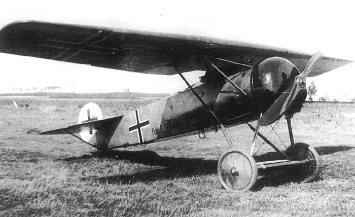
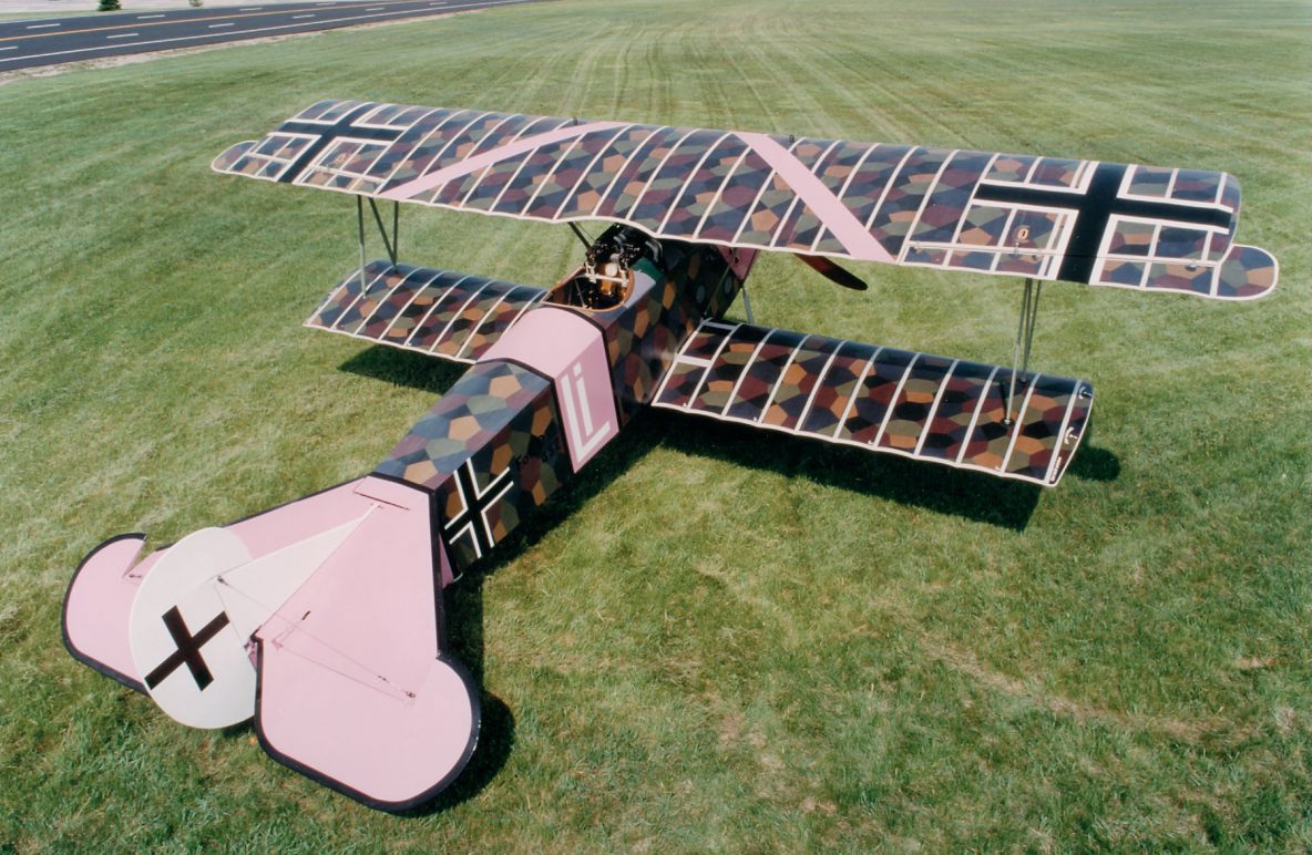
This post is a first. Up to now, all content on this blog has been exclusively written by myself. But recently Nick Mehlig and Ben Names from Structural Design and Analysis, Inc. (SDA), a team of stress engineers that design lightweight and load efficient structures, contacted me with a proposal for a guest post. The reason why I agreed is because the guys at SDA have a unique perspective on a fascinating real-world engineering problem — re-designing the wing of a Fokker D-VII. The Fokker D-VII was a German fighter aircraft in World War I but was also used by many other countries after the Great War. This post is a look at some of the details of how aircraft components are designed.

Within the Aerospace Engineering community, there is an entire sub-discipline devoted to understanding the dynamics of a system and how loads are generated (propulsive, inertial, aerodynamic, etc). In smaller companies, engineers often need to wear multiple hats, and the lines between classical stress analysis and aerodynamic loads analysis begin to blur. Recently, Structural Design and Analysis, Inc. (SDA) worked with a local resident who had taken it upon himself to build a Fokker D-VII Biplane from scratch, and wanted to know how much weight he could save if he used an aluminium spar for the main wings instead of the original wooden spar design.

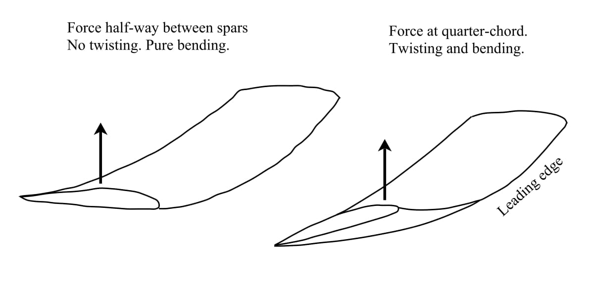
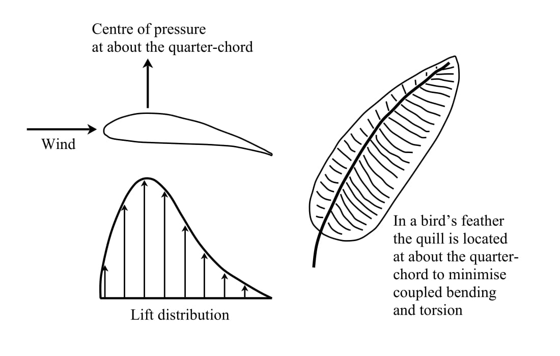
Our engineers had to develop a finite element model (FEM) and conduct the basic loads and dynamics analysis to define the load cases for the vehicle. Generating aerodynamic loads is relatively straight forward for aircraft with more conventional designs. Typically, a combination of 2D aerodynamic theory and corrections for wings with finite span are used to generate the loads in the early stages of the design phase. These loads are then applied to the structure at the quarter chord location of the wing. For the Fokker, this analysis is slightly more complicated because the biplane construction creates interference effects between the upper and lower wing which must be considered when determining the loads that act on the aircraft.

The goal of this case study is to show that various approaches can be taken to solve this loads-generation problem, and that the “best” approach for an engineer depends on his/her technical expertise, available resources (time and/or money), and the desired accuracy of the results. Three different methods were selected to calculate the aerodynamic loading on the Fokker D-VII biplane, and they are listed in increasing order of required technical expertise and accuracy:
1. Assuming that each wing can be analysed separately. This type of solution is best suited to an aircraft enthusiast or an engineer without much background in theoretical aerodynamics.
2. Accounting for the interaction between the upper and lower wing using correction factors. This type of solution is best suited for an engineer with a level of understanding comparable to an undergraduate education in aerospace engineering.
3. Using an advanced FEM analyses suite such as NX Nastran’s Static Aeroelastic SOL 144. This solution technique requires the least amount of effort on the user since the loads are calculated internally by NX Nastran, but is best suited to an engineer with some postgraduate education in aerospace engineering.
Let’s compares the efficacy of these three methods and the accuracy of their respective results.

Method 1
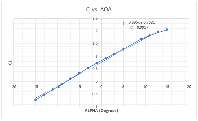
The first step in calculating the aerodynamic loads on the aircraft is to get the airfoil data. The Fokker D-VII uses a modified Goettigen GOE 418 airfoil for the upper wing. The airfoil data points (see the diagram below) were imported into XFOIL, a popular open-source 2D potential flow code, and the lift coefficients were extracted for various angles of attack (AOA). Using the XFOIL data, a plot relating the wing’s AOA to the lift coefficient ([latex] C_L [/latex]) is constructed. A trendline is added to the data to estimate the lift curve slope for the airfoil of [latex] C_{L_\alpha} = 0.095/^\circ [/latex] and the zero lift AOA is [latex]-8^\circ[/latex](the airfoil is angled down for no lift).

To calculate the lift on the upper and lower wings, a simple approximation from Prandtl Lifting Line Theory is used which relates the 3D lift coefficient to the 2D lift curve slope, the wing aspect ratio (AR) and the AOA. The lower wing of the Fokker D-VII has a [latex] 1^\circ [/latex] AOA while the upper wing has [latex] 0^\circ [/latex] AOA.

[latex] C_{L,upper} = C_{L_\alpha} \left( \frac{AR}{AR+2} \right) \left( \alpha – \alpha_{0L} \right) = 0.095 \left( \frac{5.14}{5.14+2} \right) \left( 0-(-8)\right) = 0.55 [/latex]

[latex] C_{L,lower} = C_{L_\alpha} \left( \frac{AR}{AR+2} \right) \left( \alpha – \alpha_{0L} \right) = 0.095 \left( \frac{5.67}{5.67+2} \right) \left( 1-(-8)\right) = 0.63 [/latex]

The lift equation was then used to calculate the lifting force on the wings.

[latex] L_{upper} = qS_{upper}C_{L,upper} = (0.277\ psi)(20,418.3\ in^2)(0.55) = 3,110.73\ lb [/latex]

[latex] L_{lower} = qS_{lower}C_{L,lower} = (0.277\ psi)(12,630.72\ in^2)(0.63) = 2,204.19\ lb [/latex]

where [latex] S [/latex] is the wing area and [latex] q = 1/2 \rho V^2 [/latex] is the dynamic pressure that depends on the density [latex] \rho [/latex] and the airspeed [latex] V [/latex] of the particular manoeuvre.

To balance the aircraft, the moment created by the wing lift about the centre of gravity of the Fokker needs to be balanced by the tail wing lift force, [latex] F_{tail}[/latex]. Each moment is equal to the lift force multiplied by the distance of the point of action [latex] x [/latex] from the centre of gravity of the aircraft. Given the relative positions of the two wings and the tail plane, we solve the following equation

[latex] F_{tail} = \frac{L_{lower} x_{lower} – L_{upper} x_{upper}}{x_{tail}} = \frac{3110.73 \times 11.60 – 2239.17 \times 10.41}{190.12} = 79.40\ lb [/latex]

The sum of these three loads is [latex] 3,110.73+2,204.19+79.40 = 5,394.32 [/latex] lb or 4.31g’s. Since we are analysing a 4.0g load case here, the lift on the wings will need to be reduced. As the lift on the wings is reduced, the pitching moment will change which, in turn, changes the required tail force to balance the aircraft. Excel’s goal seek was used to reduce the wing loading and balance the aircraft such that the total lift (including the tail) is equal to 4.0g. The final loads are shown below.

[latex] L_{upper} = 2,894.41 [/latex] lb

[latex] L_{lower} = 2,078.78 [/latex] lb

[latex] F_{tail} = 62.81 [/latex] lb

These final loads are applied to the quarter chord location of the wings. Here, a rectangular spanwise lift distribution is applied to the upper and lower wings.

Method 2
By having two wings subject to the same flow, each wing interacts with the other’s vortex system such that the upper wing experiences an increase in lift and the lower wing experiences a decrease in lift, denoted by [latex] \Delta C_{L,upper} [/latex] and [latex] \Delta C_{L,lower} [/latex] respectively. The following method uses the simple biplane theory which is detailed in NACA Technical Report No. 458 [1]. It is shown that the change in lift coefficient [latex] \Delta C_{L} [/latex] follows a linear relation with the overall vehicle lift coefficient [latex] C_{L} [/latex] in the following form:

[latex] \Delta C_{L,upper} = K_1 + K_2 C_L [/latex]

Where [latex] K_1 [/latex] and [latex] K_2 [/latex] are constants relating to the gap between the two wings, wing stagger (the relative fore-aft position of the two wings), decalage (angle difference between the upper and lower wings of the biplane), overhang (the extension of one wing span over the other), and wing thickness. The change in lift for the lower wing is related to the change in lift of the upper wing by the ratio of wing areas.

[latex] \Delta C_{L,lower} = -\Delta C_{L,upper} \frac{S_{upper}}{S_{lower}} [/latex]

The methods of finding the values of [latex] K_1 [/latex] and [latex] K_2 [/latex] follow a graphical approach using the biplane ratios of wing gap = 55 in., wing stagger = 25 in. , percent wing overhang = 17.4%, and decalage = 1 deg. Using these values and the method described in NACA Report 458, the following values are calculated: [latex] K_1 = -0.090 [/latex] and [latex] K_2 = 0.195 [/latex]. The final lift coefficient for the upper and lower wings are found by adding the correction to the vehicle lift coefficient to the original uncorrected value. This uncorrected value is calculated from the maximum weight of the aircraft, which naturally determines the lift required from the wings. The maximum weight of the Fokker D-VII is 1,259 lbs, and for a 4.0g manoeuvre (n=4 in the equation below), the aircraft lift coefficient is:

[latex] C_L = \frac{nW}{0.5 \rho V^2 S} = \frac{nW}{qS} = \frac{4 \times 1259}{0.277 \times 33049} = 0.55 [/latex]

Plugging in values for [latex] K_1 [/latex], [latex] K_2 [/latex] and [latex] C_L [/latex] into the [latex] \Delta C_{L,upper}[/latex] and [latex] \Delta C_{L,lower}[/latex] equations give the following values:

[latex] \Delta C_{L,upper} = 0.015 [/latex] and [latex] \Delta C_{L,lower} = -0.025 [/latex]

Using the new corrected values for the wing coefficients [latex] C_{L,upper} = C_L + \Delta C_{L,upper}[/latex] and [latex] C_{L,lower} = C_L + \Delta C_{L,lower}[/latex], the total load can be calculated for the upper and lower wings. A moment balance is performed and the following loads are calculated for the aircraft:

[latex] L_{upper} = 3,139.88 [/latex] lb

[latex] L_{lower} = 1,803.24[/latex] lb

[latex] F_{tail} = 92.87[/latex] lb

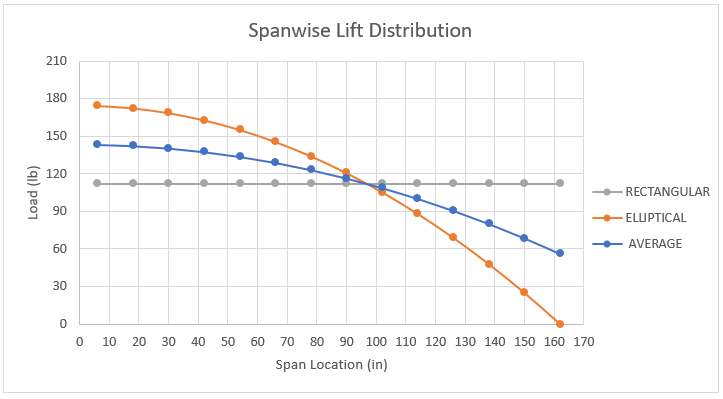
Again, the loads are applied to the quarter-chord position of the aircraft wings. Two different spanwise lift distributions are applied to the model for this comparison study. The first assumes an elliptical lift distribution. The second uses Schrenk’s Approximation to estimate a more accurate spanwise lift distribution. These two distributions are shown below along with a reference to a rectangular distribution.

Method 3
The third and final method is to use NX Nastran’s static aeroelastic SOL 144 analysis to generate the loads using a vortex lattice formulation. A potential flow model is created in FEMAP to generate the aerodynamic loading for the Fokker. One of the powerful functionalities about SOL 144 trim analysis is that given high-level information about any flight condition, Nastran cannot only calculate the aerodynamic forces, but can also ensure that the vehicle is stable. With just a few clicks, the load case can be modified to model any corner of the flight envelope by changing the dynamic pressure and load factor of the aircraft. Since Nastran calculates all the loads internally using this high-level flight condition information, it can save an incredible amount of time that might be devoted to calculating loads externally, bringing them in, and applying them to the structure accurately. This solution requires the least amount of effort on the user since the loads are calculated internally by NX Nastran and then applied to the FEM through the points defined in the model. NX Nastran automatically calculates the trim condition of the aircraft and calculates the loading on the upper wing, lower wing, and horizontal tail. The resulting loads are shown below:

[latex] L_{upper} = 3223.21 [/latex] lb

[latex] L_{lower} = 1,697.10[/latex] lb

[latex] F_{tail} = 122.75 [/latex] lb

Results
As the complexity increases with each of the methods discussed above, so does the accuracy of the results. However, not every stage of the design requires the same precision. Since this discussion focuses on how the analysis approach impacts the design of the aircraft, let us first compare the calculated loads for all three methods. Below is a table outlining the loads for each method and the percentage difference when compared to the aeroelasticity finite element model (the most accurate loads generation approach).

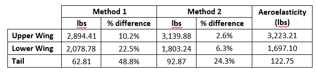
When comparing the lifting force of upper and lower wings of the aircraft, the aerodynamic loading from method 1 underestimates the lift on the upper wing by 10.2% and over estimates the lift on the lower wing by 22.5%. Applying Simple Biplane Theory in method 2 captures the interference effects and estimates the wing loading much more accurately with the upper wing lift only 2.6% less and the lower wing lift 6.3% greater, when compared to the aeroelastic model. A more detailed way to compare the resulting design impact of the three different load generation methods is to look at the internal shear and bending moment diagrams within the spars. Below is the shear force diagram for the upper wing leading edge spar.

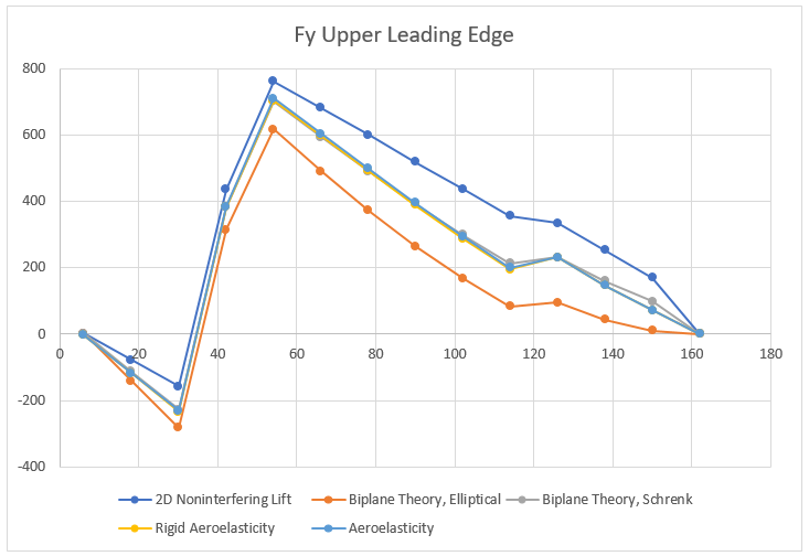
Starting with the simplest method, the 2D non-interfering lift generates the highest shear force. As one would expect the variation in the maximum internal shear force is small (at most 7% difference) over all the models since the total lift generated by the plane was set to be constant. The differences are partially due to how the lift is distributed between the upper and lower wings. Furthermore, the spanwise distribution clearly has an impact on the internal shear force. Interestingly, the model that matches the shear force of the aeroelasticity model the closest is the Biplane Theory model using Schrenk’s approximation. The differences produced by these aerodynamic models becomes even more apparent when inspecting the internal bending moment.

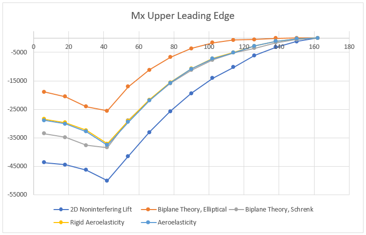
The internal bending moment clearly shows how differences in the aerodynamic models can propagate. The most basic model (2D Non-interfering Lift) produces the highest bending moment, 33% higher than the aeroelastic solution. While it is safer to be on the conservative side, this kind of inaccuracy will lead to a substantially heavier structure, thus limiting performance.

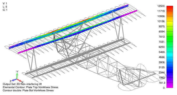
The shear and bending moment diagrams are often excellent indicators of the internal stress state within simple structures. As a stress engineer, comparing stress plots is the most meaningful way to compare how the different aerodynamics models impact the stress throughout the vehicle. Below is a picture of the upper wing leading and trailing edge spars Von Mises stress under a 4g pull up when using the aeroelasticity model.

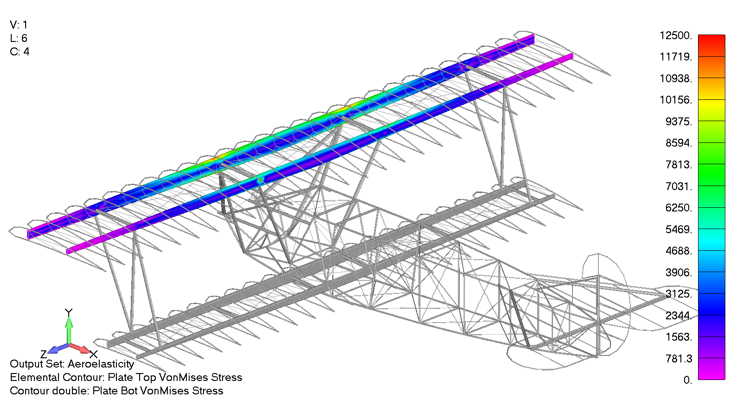
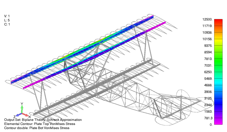
The max spar cap Von Mises stress is 11.4 ksi. In comparison, the same stress contour is presented below, only for the case using the Biplane theory using Schrenk’s approximation, which exhibited a maximum Von Mises stress of 11.5 ksi, a 0.8% difference from the aeroelastic aerodynamic model.

In contrast, the Von Mises stress state for the upper wing under the 2D non-interfering lift can be seen below as a gross overprediction, predicting a maximum Von Mises stress of 15.2 ksi, 33% higher than the aeroelastic aerodynamic model.

Conclusion
Having exhaustively explored the impact of different aerodynamic models on the final stress results, several conclusions have become clear. First and foremost, as laid out at the beginning, none of these approaches are inherently bad. However their mileage does vary significantly. Requiring the least technical background, the 2D non-interfering lift model provides a good approximation of the stress state in the leading and trailing edges, but is over-conservative in predicting internal stresses. As expected, including the interference effects between the upper and lower wing in the simple Biplane Theory and applying finite span effects has the potential to predict stresses within 0.8% of the most accurate model. Unfortunately, this relies on the user correctly calculating the span wise loading and interference effects which often requires complex analytical methods or using a potential flow method. Furthermore, there are ample opportunities for an engineer to make a mistake when taking this approach, and it could be difficult to detect these without the results of a more accurate model to compare to.

Now, given that fairly accurate stress distributions using semi-analytical methods can be achieved, you might be asking yourself, why might anyone want to spend the money to use the NX Nastran Aeroelasticity module? First, it removes substantial uncertainty in the accuracy of the aerodynamic model. The Nastran Aeroelasticity module can account for interfering lifting surfaces, slender fuselage effects, ground effect, compressibility, wing sweep and taper, as well as a number of other factors. Additionally, once implemented, the Nastran Aeroelasticity module is more flexible than generating the loads from an outside source and then applying those loads within FEMAP (the pre/post environment). Nastran can generate the loads for any flight condition such as steady level flight, a 4g pull up, or a 3g coordinated turn, requiring only high level information from the user.

Finally, the user is also provided with additional information such as the trim angle of attack, control surface deflection angles, and vehicle stability derivatives. As with most problems, there is rarely a single correct approach, but when high accuracy and case-generation flexibility are desired, then using NX Nastran’s Static Aeroelastic Solution 144 is the way to go. However, if you are working on a budget, can take on additional mass, or do not have the technical background to employ Solution 144, then using an analytical method or generating the loads some other way externally is probably the way to go.

References

[1] Diehl, W. S., “Relative Loading on Biplane Wings,” NACA TR-458, January 1934
June 26, 2017
Why are aircraft not made of glass?

J.E. Gordon, a leading engineer at the Royal Aircraft Establishment at Farnborough and holder of the British Silver Medal of the Royal Aeronautical Society, wrote two brilliant books on engineering: “The New Science of Strong Materials” and “Structures – Or Why Things Don’t Fall Down”. Elon Musk has recommended the latter of the two books, and I can only encourage you to read both. In my eyes, the role of a good non-fiction writer is to explain the intricacies of a non-trivial topic that we can see all around us but nevertheless rarely fully appreciate. Something interesting hidden in plain sight, if you will.

With this in mind, let’s discuss an underappreciated topic from the world of materials science.

First of all, what do we mean by a material’s stiffness and strength?

To be able to compare the load and deformation acting on components of different sizes, engineers prefer to use the quantities of stress and strain over load and deformation. Imagine a solid rod of a certain diameter and length which is being pulled apart in tension. Naturally, two rods of the same material but of different diameters and lengths will deform by different amounts. However, if both rods are stressed by the same amount, then they will experience the same amount of strain. In our simple one-dimensional rod example, the stress [latex] \sigma [/latex] is given by

[latex] \sigma = \frac{P}{A} [/latex]

where [latex]P[/latex] is the tensile force and [latex]A = \pi d^2 / 4[/latex] is the cross-sectional area for a diameter [latex] d [/latex], i.e. force normalised by cross-sectional area.

The engineering strain [latex] \epsilon [/latex] is given by

[latex] \epsilon = \frac{\Delta L}{L} [/latex]

where [latex]\Delta L[/latex] is the change in length (deformation) of the rod and [latex]L[/latex] is its original length, i.e. the deformation normalised by original length.

For an elastic material deforming linearly (i.e. no plastic deformation), the ratio of stress to strain is constant, and for our simple one-dimensional example the constant of proportionality is equal to the stiffness of the material.

[latex] E = \frac{\sigma}{\epsilon} [/latex] (Hooke’s Law).

This stiffness [latex] E [/latex] is known as the Young’s modulus of the material.

These two definitions of stress and strain illustrate a simple point. By dividing force by cross-sectional area and change in length (deformation) by original length, the role of geometry is eliminated entirely. This means we can deal purely in terms of material properties, i.e. Young’s modulus (stiffness), stress to failure (strength), etc., and can therefore compare the degree of loading (stress) and deformation (strain) in components of different sizes, shapes, dimensions, etc.

We can all appreciate that metals are incredibly strong and stiff. But why are some materials stronger and stiffer than others? Why don’t all materials have the same strength and stiffness? Aren’t all materials just an assemblage of molecules and atoms whose molecular bonds stretch and eventually separate upon fracture? If this is so, why don’t all materials break at the same value of stress and strain?

The stiffness and strength of a material does indeed depend on the relative stiffness and strength of the underlying chemical bonds, and these do vary from material to material. But this difference is not sufficient to explain the large variations in strength that we observe for materials such as steel and glass – that is, why does glass break so easily and steel does not?

In the 1920s, a British engineer called A.A. Griffith explained for the first time why different materials have such vastly different strengths. To calculate the theoretical maximum strength of a material, we need to use the concept of strain energy. When we stretch a rod by 1 mm using a force of 1,000 N, the 1 J of energy we exerted (0.001 m times 1,000 N) is stored within the material as strain energy because individual atomic bonds are essentially stretched like mechanical springs. Written in terms of stresses and strains, the strain energy stored within a unit volume of material is simply half the product of stress and strain:

[latex] \text{Strain Energy per unit volume} = \frac{1}{2} \sigma \times \epsilon [/latex]

Griffith’s brilliant insight was to equate the strain energy stored in the material just before fracture to the surface energy of the two new surfaces created upon fracture.

Surface energy??

It is probably not immediately obvious why a surface would possess energy. But from watching insects walk over water we can observe that liquids must possess some form of surface tension that stops the insect from breaking through the surface. When the surface of a liquid is extended, say by inflating a soap bubble, work is done against this surface tension and energy is stored within the surface. Similarly, when an insect is perched on the surface of a pond, its legs form small dimples on the surface of the water and this deformation causes an increase in the surface energy. In fact, we can calculate how far the insect sinks into the surface by equating the increase in surface energy to the decrease in gravitational potential energy as the insect sinks. Furthermore, liquids tend to minimise their surface energy under the geometrical and thermodynamic constraints placed upon them, and this is precisely why raindrops are spherical and not cubic.

When a liquid freezes into a solid, the underlying molecular structure changes, but the overall surface energy remains largely the same. Because the molecular bonds in solids are so much stronger than those in liquids, we can’t actually see the effect of surface tension in solids (an insect landing on a block of ice will not visibly dimple the external surface). Nevertheless, the physical concept of surface energy is still valid for solids.

So, back to our fracture problem. What we want to calculate is the stress which will separate two adjacent rows of molecules within a material. If the rows of molecules are initially [latex] d [/latex] metres apart then a stress [latex] \sigma [/latex] causing a strain [latex] \epsilon [/latex] will lead to the following strain energy per square metre

[latex] \text{Strain Energy per unit area} = \frac{1}{2} \sigma \times \epsilon \times d[/latex]

From Hooke’s law we know that

[latex] \epsilon = \frac{\sigma}{E} [/latex]

and therefore replacing [latex]\epsilon[/latex] in the first equation we have

[latex] \text{Strain Energy per unit area} = \frac{d\sigma^2}{2E}[/latex]

Now, if the surface energy per square metre of the solid is equal to [latex]G[/latex], then the separation of the two rows of molecules will lead to an increase in surface energy of [latex]2G[/latex] (two new surfaces are created). By assuming that all of the strain energy is converted to surface energy:

[latex] \frac{d\sigma^2}{2E} = 2G \Rightarrow \sigma = 2 \sqrt{\frac{G E}{d}}[/latex]

There is typically a considerable amount of plastic deformation in the material before the atomic bonds rupture. This means that the Young’s modulus decreases once the plastic regime is reached and the strain energy is roughly half of the ideal elastic case. Hence, we can simply drop the 2 in front of the square root above to get a simple, yet approximate, expression for the strength of a material

[latex] \sigma = \sqrt{\frac{G E}{d}}[/latex]

As the values of [latex] E [/latex] and [latex] G [/latex] vary from material to material, the theoretical strengths will be different as well. The surface tension of a material is roughly proportional to the Young’s modulus because the same chemical bonds give rise to both these properties. In fact, the relationship between surface energy and Young’s modulus can be approximated as

[latex] G \approx \frac{Ed}{20}[/latex]

such that the strength of a material is approximately proportional to the Young’s modulus by the following relation

[latex] \sigma \approx \sqrt{\frac{E^2}{20}} \approx \frac{E}{5}[/latex]

Given, the relationship between stress and strain we can conclude that the theoretical failure strain of most materials ought to be, approximately,

[latex] \epsilon = \frac{\sigma}{E} \approx \frac{1}{5}[/latex]

or 20% for basically all materials.

In everyday practise, most materials have failure strengths far beneath the theoretical maximum and also vary widely in their failure strains. To explain why, Griffith conducted some simple experiments on glass. After calculating the Young’s modulus [latex] E [/latex] from a simple tensile test and assuming a molecular spacing of [latex] d = 3 [/latex] Angstroms, Griffith arrived at a theoretical strength for glass of 14,000 MPa. Griffith then tested a number of 1 mm diameter glass rods in tension and found the strength to be on average around 170 MPa, i.e. [latex] 1/100 [/latex]th of the theoretical value.

The pultrusion process used to create the glass rods allowed Griffith to pull thinner and thinner rods, and as the diameter decreased, the failure stress of the rods started to increase – slowly at first, but then very rapidly. Glass fibres of 2.5 [latex]\mu[/latex]m in diameter showed strengths of 6,000 MPa when newly drawn, but dropped to about half that after a few hours. Griffith was not able to manufacture smaller rods so he fitted a curve to his experimental data and extrapolated to much smaller diameters. And lo and behold, the exponential curve converged to a failure strength of 11,000 MPa – much closer to the 14,000 MPa predicted by his theory.

Variation of tensile strength with fibre diameter. From W.H. Otto (1955). Relationship of Tensile Strength of Glass Fibers to Diameter. Journal of the American Ceramic Society 38(3): 122-124.

Griffith’s next goal was to explain why the strength of thicker glass rods fell so far below the theoretical value. Griffith surmised that as the volume of a specimen increases, some form of weakening mechanisms must be active because the underlying chemical structure of the material remains the same. This weakening mechanism must somehow lead to an increase in the actual stress around a future failure site and act as a stress concentration. Luckily, the idea of stress concentrations had previously been introduced in the naval industry, where the weakening effects of hatchways and other openings in the hull had to be accounted for. Griffith decided that he would apply the same concept at a much smaller scale and consider the effects of molecular “openings” in a series of chemical bonds.

The idea of a stress concentration is quite simple. Any hole or sharp notch in a material causes an increase in the local stress around the feature. Rather counter-intuitively, the increase in local stress is solely a function of the shape of the notch and not of its size. A tiny hole will weaken the material just as much as a large one will. This means a shallow cut in a branch will lower the load-carrying capacity just as well as a deep one – it is the sharpness of the cut that increases the stress.

We can visualise quite easily what must happen at a molecular scale when we introduce a notch in a series of molecules. A single strand of molecules must reach the maximum theoretical strength. Similarly, placing a number of such strands side by side should not effect the strength. However, if we cut a number of adjacent strands at a specific location perpendicular to the loading direction, then the flow of stress from molecule to molecule has been interrupted and the load in the material has to be redistributed to somewhere else. Naturally, the extra load simply goes around the notch and will therefore have to pass through the first intact bond. As a result, this bond will fail much earlier than any of the other bonds as the stress is concentrated in this single bond. As this overloaded bond breaks, the situation becomes slightly worse because the next bond down the line has to carry the extra load of all the broken bonds.

Stress concentration at a notch

The stress concentration factor of a notch of half-length [latex] a [/latex] and radius of curvature at the crack tip [latex] R [/latex] is given by

[latex] 1 + 2 \sqrt{\frac{a}{R}} [/latex]

If we now consider a crack about 2 [latex]\mu[/latex]m long and 1 Angstrom tip radius, this produces a stress concentration factor of

[latex] 1 + 2 \sqrt{\frac{1 \times 10^{-6}}{1 \times 10^{-10}}} = 201 [/latex]

and therefore this would lower the theoretical strength of glass from 14,000 MPa to around 70 MPa, which is very close to the average strength of typical domestic glass.

As a result, Griffith made the conjecture that glass and all other materials are full of tiny little cracks that are too small to be seen but nevertheless significantly reduce the theoretical maximum strength. Griffith did not give an explanation for why these cracks appeared in the first place or why they were rarer for thinner glass rods. As it turns out, Griffith was correct about the mechanism of stress concentrationa, but wrong about their origins.

It took quite some time until a more satisfactory explanation was provided, dispelling the notion that the reduction in strength could be attributed to inherent defects within the material. After WWII, experiments showed that even thick glass rods could approach the theoretical upper limit of strength when carefully manufactured. It was also noticed that stronger fibres would weaken over time, probably as a result of handling, and that weakened fibres could consequently be strengthened again by chemically removing the top surface. By depositing sodium vapour on the external surface of glass, the density of cracks could be visualised and was found to be inversely proportional to the strength of the glass – the more cracks, the lower the strength, and vice versa.

These cracks are a simple result of scratching when the exterior surface comes in contact with other objects. Larger pieces of glass are more likely to develop surface cracks due to the larger surface area. Furthermore, thin glass fibres are much more likely to bend when in contact with other objects, and are therefore less likely to scratch. This means that there is nothing special about thin fibres of glass – if the surface of a thick fibre can be kept just as smooth as that of a thin fibre then it will be just as strong.

This means that an airplane cast from one piece of 100% pristine glass could theoretically sustain all flight loads, such an idea ludicrous in reality, because the likelihood of inducing surface cracks during service is basically 100%.

At this point you might be asking, what is different about metals – why are they used on aircraft instead?

The difference boils down to differences between the atomic structure of glasses and metals. When liquids freeze they typically crystallise into a densely packed array and form a solid that is denser than the liquid. Glasses on the other hand do not arrange themselves into a nicely packed crystalline structure but rather cool into a purely solidified liquid. Glasses can crystallise under some circumstances under a process known as devitrification, but the glass is often weakened as a result. When a solid crystallises, it can deform via a new process in which it starts to flow in shear just like Plasticine or moulding clay does when it is formed.

There is no clear demarcation line between a brittle (think glass) and ductile (think metal) material. The general rule of thumb is that a brittle material does not visibly deform before failure and failure is caused by a single crack that runs smoothly through the entire material. This is why it’s often possible to glue a broken vase back together.

In ductile materials, there is permanent plastic deformation before ultimate failure and so these materials behave more like moulding clay. Before a ductile material, like mild steel, finally snaps in two, there is considerable plastic deformation which can be imagined along the lines of flowing honey or treacle. This plastic flowing is caused by individual layers of atoms sliding over each other, rather than coming apart directly. As this shearing of atomic bonds takes place, the material is not significantly weakened because the atomic bonds have the ability to re-order, and the material may even be strengthened by a process known as cold working (atomic bonds align with the direction of the applied load). The amount of shearing before final failure depends largely on the type of metal alloy and always increases as a metal is heated; hence a blacksmith heats metal before shaping it.

Generally, these two fracture mechanism, brittle cracking and plastic flowing, are always competing in a solid. The material will break in whatever mechanism is weakest; yield before cracking if it is ductile or crack directly if it is brittle.

March 18, 2017
From Wright Flyer to Space Shuttle
On December 17 1903, the bicycle mechanic Orville Wright completed the first successful flight in a heavier-than-air machine. A flight that lasted a mere 12 seconds, reaching an altitude of 10 feet and landing 120 feet from the starting point. The Wright Flyer was made of wood and canvas, powered by a 12 horsepower internal combustion engine and endowed with the first, yet basic, mechanisms for controlling pitch, yaw and roll. Only 66 years later, Neil Armstrong walked on the moon, and another 12 years later the first partially re-usable space transportation system, the Space Shuttle, made its way into orbit.

Even though the means of providing lift and attitude control in the Wright Flyer and the Space Shuttle were nearly identical, the operational conditions could not be more different. The Space Shuttle re-entered the atmosphere at orbital velocity of 8 km/s (28x the speed of sound), which meant that the Shuttle literally collided with the atmosphere, creating a hypersonic shock wave with gas temperatures close to 12,000°C -temperature levels hotter than the surface of the sun. How was such unprecedented progress – from Wright Flyer to Space Shuttle – possible in a mere 78 years? This blog post chronicles this technological evolution by telling the story of five iconic aircraft.

The Wright brothers were the first to succesfully fly what we now consider a modern airplane, but as the brothers would adamantly confirm, they did not invent the airplane. Rather, the brothers stood on the shoulders of a century-old keen interest in aeronautical research. The story of the modern airplane goes back to about 100 years before the Wright brothers, to a relatively unknown British scientist, philosopher, engineer and member of parliament, Sir George Cayley. Although Leonardo da Vinci had thought up flying machines 300 years prior to this, his inventions have relatively little in common with modern designs. In 1799 Cayley proposed the first three-part concept that, to this day, represent the fundamental operating principles of flying:
- A fixed wing for creating lift.
- A separate mechanism using paddles to provide propulsion.
- And a cruciform tail for horizontal and vertical stability.
Many of the flying enthusiasts of the 18th century based their designs on the biomimicry of birds, combining lift, propulsive and control functions in a single oversized wing contraption that was insufficient at providing lift, forward propulsion, let alone a means of control. During a decade of intensive study of the aerodynamics of birds and fish from 1799-1810, Cayley constructed a series of rotating airfield apparatuses that tested the lift and drag of different airfoil shapes. In 1852, Cayley published his most famous work “Sir George Cayley’s Governable Parachutes”, which detailed the blueprint of a large glider with almost all of the features we take for granted on a modern aircraft. A prototype of this glider was built in 1853 and flown by Cayley’s coachman, accelerating the prototype off the rooftop of Cayley’s house in Yorkshire.

The distinctive characteristic of the Wright brothers was their incessant persistence and never-ending scepticism of the research conducted by scientists of authority. By single-handedly revising the historic textbook data on airfoils and building all of their inventions themselves, they developed into the most experienced aeronautical engineers of their day. Engineering often requires a certain intuitive knowledge of what works and what doesn’t, typically acquired through first-hand experience, and the Wright brothers had developed this knack in abundance. In this sense, they were best-equipped to refine the concepts of their peers and develop them into something that superseded everything that came before.

One of the most potent signals of British defiance in WWII is the Supermarine Spitfire. In the summer of 1940, during the Battle of Britain, the Spitfire presented the last bulwark between tyranny and democracy. Between July and October 1940, 747 Spitfires were built of which 361 were destroyed and 352 were damaged. Just 34 Spitfires that were built during the summer of 1940 made it through the war unscathed. Unsurprisingly, the Spitfire is one of the most famous airplanes of all time and its aerodynamic beauty of elliptical wings and narrow body make it one of the most iconic aircraft ever built.

The Spitfire was designed by the chief engineer of Supermarine, RJ Mitchell. Before WWII Mitchell led the construction of a series of sea-landing planes that won the Schneider Trophy three times in a row in 1927, 1929 and 1931. The Schneider Trophy was the most important aviation competition between WWI and WWII – initially intended to promote technical advances in civil aviation, it quickly morphed into pure speed contest over a triangular course of around 300 km. As competitions so often do, the Schneider Trophy became an impetus for advancing aeroplane technology, particularly in aerodynamics and engine design. In this regard the Schneider Trophy had a direct impact on many of the best fighters of WWII. The low drag profile and liquid-cooled engine which were pioneered during the Schneider Trophy were all features of the Supermarine Spitfire and the Mustang P-51. The winning airplane in 1931 was the Supermarine S6.B, setting a new airspeed record of 655.8 km/h (407.4 mph). The S6.B was powered by the supercharged Rolls-Royce R engine with 1900 bhp, which presented such insurmountable problems with cooling that surface radiators had to be attached to the buoyancy floats used to land on water. In March 1936, Mitchell evolved the S6.B into the Spitfire with a new Rolls Royce Merlin engine. The Spitfire also featured its radical elliptical wing design which promised to minimise lift-induced drag. Theoretically, an infinitely long wing of constant chord and airfoil section produces no induced drag. A rectangular wing of finite length however produces very strong wingtip vortices and as a result almost all modern wings are tapered towards the tips or fitted with wing tip devices. The advantage of an elliptical planform (tapered but with curved leading and trailing edges) over a tapered trapezoidal planform is that the effective angle of attack of the wing can be kept constant along the entire wingspan. Elliptical wings are probably a remnant of the past as they are much more difficult to manufacture and the benefit over a trapezoidal wing is negligible for the long wing spans of commercial jumbo jets. However, the design will forever live on in one of the most iconic fighters of all time, the Supermarine Spitfire.

Captain Chuck Yeager, an American WWII fighter ace, became the first supersonic pilot in 1947 when the chief test pilot for the Bell Corporation refused to fly the rocket-powered Bell X-1 experimental aircraft without any additional danger pay. The X-1 closely resembled a large bullet with short stubby wings for higher structural efficiency and less drag at higher speeds. The X-1 was strapped to the belly of a B-29 bomber and then dropped at 20,000 feet, at which point Yeager fired his rocket motors propelling the aircraft to Mach 0.85 as it climbed to 40,000 feet. Here Yeager fully opened the throttle, pushing the aircraft into a flow regime for which there was no available wind tunnel data, ultimately reaching a new airspeed record of Mach 1.06. Yeager had just achieved something that had eluded Europe’s aircraft engineers through all of WWII.

The limit that the European aircraft designer ran into during the air speed competitions prior to WWII was the sound barrier. The problem of flying faster, or in fact approaching the speed of sound, is that shock waves start to form at certain locations over the aircraft fuselage. A shock wave is a thin front (about 10 micrometers thick) in which molecules are squashed together by such a degree that it is energetically favourable to induce a sudden increase in the fluid’s density, temperature and pressure. As an aircraft approaches the speed of sound, small pockets of sonic or supersonic flow develop on the top surface of the wing due to airflow acceleration over the curved upper skin. These supersonic pockets terminate in a shockwave, drastically slowing the airflow and increasing the fluid pressure. Even in the absence of shock waves the airflow runs into an adverse pressure gradient towards the trailing edge of the wing, slowing the airflow and threatening to separate the boundary layer from the wing. This condition drastically increases the induced drag and reduces lift, which in the worst case can lead to aerodynamic stall. In the presence of a shock wave this scenario is exacerbated by the sudden increase in pressure and drop in airflow velocity across the shock wave. For this precise reason, commercial aircraft are limited to speeds of around Mach 0.87-0.88 as any further increase in speed would induce shock waves over the wings, increasing drag and requiring an unproportional amount of additional engine power.

It was precisely this problem that aircraft designers ran into in the 1930’s and 1940’s. To make their airplanes approach the speed of sound they needed incredible amounts of extra power, which the internal combustion engines of the time could not provide. Quite fittingly this seemingly insurmountable speed limit was dubbed the sound barrier. It was not until the advent of refined jet engines after WWII that the sound barrier was broken. However, exceeding the sound barrier does not mean things get any easier. The ratio of upstream to downstream airflow speed and pressure across a shock wave are simple functions of the upstream Mach number (airspeed / local speed of sound). Unfortunately for aircraft designers, these ratios change with the square of the upstream Mach number, which means that the induced drag becomes worse and worse the further the speed of sound is exceeded. This is why the Concorde needed such powerful engines and why its fuel costs were so exorbitant.

The North American X-15 rocket plane was one of NASA’s most daring experimental aircraft intended to test flight conditions at hypersonic speeds (Mach 5+) at the edge of space. Three X-15s made 199 flights from 1960-1968 and the data collected and knowledge gained directly impacted the design of the Space Shuttle. Initially designed for speeds up to Mach 6 and altitudes up to 250,000 feet, the X-15 ultimately reached a top speed of Mach 6.72 (more than one mile a second) and a maximum altitude of 354,200 feet (beyond the official demarcation line of space). As of this writing, the X-15 still holds the world record for the highest speed recorded by a manned aircraft. Given the awesome power required to overcome the induced drag of flying at these velocities, it is no surprise that the X-15 was not powered by a traditional turbojet engine but rather a full-fledged liquid-propellant rocket engine, gulping down 2,000 pounds of ethyl alcohol and liquid oxygen every 10 seconds.

The X-15 was dropped from a converted B-52 bomber and then made its way on one of two different experimental flight profiles. High-speed flights were conducted at an altitude of a typical commercial jetliner (below 100,000 feet) using conventional aerodynamic control surfaces. For high-altitude flights the X-15 initiated a steep climb at full throttle, followed by engine shut-down once the aircraft left Earth’s atmosphere. What followed was a ballistic coast, carrying the aircraft up to the peak of an arc and then plummeting back to Earth. Beyond Earth’s atmosphere the aerodynamic control surfaces of the X-15 were obviously useless, and so the X-15 relied on small rocket thrusters for control.

The hypersonic speeds beyond the conventional sound barrier discussed previously created a new problem for the X-15. In any medium, sound is transmitted by vibrations of the medium’s molecules. As an aircraft slices through the air, it disturbs the molecules around it which ensues in a pressure wave as molecules bump into adjacent molecules, sequentially passing on the disturbance. Flying faster than the speed of sound means that the aircraft is moving faster than this pressure wave. Put another way, the air molecules are transmitting the information of the disturbance created by the aircraft via a pressure wave that travels at the speed of sound. While the aircraft is creating new disturbances further upstream, Nature can’t keep up with the aircraft. At hypersonic speeds the aircraft is literally smashing into the surrounding stationary air molecules, and the ensuing compression of the air around the aircraft skin leads to fluid temperatures that are above the melting point of steel. Hence, one of the major challenges of the X-15 was guaranteeing structural integrity at these incredibly high temperatures. As a result, the X-15 was constructed from Inconel X, a high-temperature nickel alloy, which is also used in the very hot turbine stages of a jet-engine.

The wedge tail visible at the back of the aircraft was also specifically required to guarantee attitude stability of the aircraft at hypersonic speeds. At lower speeds this thick wedge created considerable amounts of drag, in fact as much as some individual fighter aircraft alone. The area of the tail wedge was around 60% of the entire wing area and additional side panels could be extended out to further increase the overall surface area.

12 April 1981 marked a new era in manned spaceflight: Space Shuttle Columbia lifted off for the first time from Cape Canaveral. The Shuttle capped an incredible fruitful period in aerospace engineering development. The ground work laid by the original Wright flyer, the Spitfire, the X-1 and the X-15 is all part of the technological arc that led to the Shuttle. The fundamentals didn’t change but their orders of magnitude did.

“Like bolting a butterfly onto a bullet” — Story Musgrave, Columbia astronaut, 1996

Story Musgrave’s description of the Space Shuttle is not far off the mark. On the launch pad the Shuttle sat on two solid-rocket boosters producing 37 million horsepower, accelerating the Shuttle beyond the speed of sound in about 30 seconds. Eight minutes and 500,000 gallons of fuel later the Shuttle was travelling at 17,500 mph at the edge of space. The Space Shuttle was not only powerful but possessed a grace that the Wright brothers would have appreciated. After smashing through the atmosphere upon reentry at Mach 28 (8 km/s) the piloting astronaut had to slow the Shuttle down to 200 mph via a series of gliding twists and turns, using the surrounding air as an aerodynamic break.

The ultimate mission of the Shuttle was to serve as a cost-effective means of travelling to space for professional astronauts and civilians. That vision never came to fruition due to the high maintenance costs between flights, and partly due the Challenger and Columbia disasters that shattered all hopes that space travel would become routine.

Perhaps the Space Shuttle is one of humanities greatest inventions because it reminds us that for all its power, grace and genius it is still the brainchild of fallible men.

Edits:

A previous version of this article incorrectly stated that the Space Shuttle featured three solid rocket boosters (SRBs). Of course, the Space Shuttle only featured two.
February 15, 2017
Boundary Layer Separation and Pressure Drag
At the start of the 19th century, after studying the highly cambered thin wings of many different birds, Sir George Cayley designed and built the first modern aerofoil, later used on a hand-launched glider. This biomimetic, highly cambered and thin-walled design remained the predominant aerofoil shape for almost 100 years, mainly due to the fact that the actual mechanisms of lift and drag were not understood scientifically but were explored in an empirical fashion. One of the major problems with these early aerofoil designs was that they experienced a phenomenon now known as boundary layer separation at very low angles of attack. This significantly limited the amount of lift that could be created by the wings and meant that bigger and bigger wings were needed to allow for any progress in terms of aircraft size. Lacking the analytical tools to study this problem, aerodynamicists continued to advocate thin aerofoil sections, as there was plenty of evidence in nature to suggest their efficacy. The problem was considered to be more one of degree, i.e. incrementally iterating the aerofoil shapes found in nature, rather than of type, that is designing an entirely new shape of aerofoil in accord with fundamental physics.

During the pre-WWI era, the misguided notions of designers was compounded by the ever-increasing use of wind-tunnel tests. The wind tunnels used at the time were relatively small and ran at very low flow speeds. This meant that the performance of the aerofoils was being tested under the conditions of laminar flow (smooth flow in layers, no mixing perpendicular to flow direction) rather than the turbulent flow (mixing of flow via small vortices) present over the wing surfaces. Under laminar flow conditions, increasing the thickness of an aerofoil increases the amount of skin-friction drag (as shown in last month’s post), and hence thinner aerofoils were considered to be superior.

The modern plane – born in 1915

The situation in Germany changed dramatically during WWI. In 1915 Hugo Junkers pioneered the first practical all-metal aircraft with a cantilevered wing – essentially the same semi-monocoque wing box design used today. The most popular design up to then was the biplane configuration held together by wires and struts, which introduced considerable amounts of parasitic drag and thereby limited the maximum speed of aircraft. Eliminating these supporting struts and wires meant that the flight loads needed to be carried by other means. Junkers cantilevered a beam from either side of the fuselage, the main spar, at about 25% of the chord of the wing to resist the up and down bending loads produced by lift. Then he fitted a smaller second spar, known as the trailing edge spar, at 75% of the chord to assist the main spar in resisting fore and aft bending induced by the drag on the wing. The two spars were connected by the external wing skin to produce a closed box-section known as the wing box. Finally, a curved piece of metal was fitted to the front of the wing to form the “D”-shaped leading edge, and two pieces of metal were run out to form the trailing edge. This series of three closed sections provided the wing with sufficient torsional rigidity to sustain the twisting loads that arise because the centre of pressure (the point where the lift force can be considered to act) is offset from the shear centre (the point where a vertical load will only cause bending and no twisting). Junker’s ideas were all combined in the world’s first practical all-metal aircraft, the Junker J 1, which although much heavier than other aircraft at the time, developed into the predominant form of construction for the larger and faster aircraft of the coming generation.

Junkers J 1 at Döberitz in 1915
Structures + Aerodynamics = Superior Aircraft

Junkers construction naturally resulted in a much thicker wing due to the room required for internal bracing, and this design provided the impetus for novel aerodynamics research. Junker’s ideas were supported by Ludwig Prandtl who carried out his famous aerodynamics work at the University of Göttingen. As discussed in last month’s post, Prandtl had previously introduced the notion of the boundary layer; namely the existence of a U-shaped velocity profile with a no-flow condition at the surface and an increasing velocity field towards the main stream some distance away from the surface. Prandtl argued that the presence of a boundary layer supported the simplifying assumption that fluid flow can be split into two non-interacting portions; a thin layer close to the surface governed by viscosity (the stickiness of the fluid) and an inviscid mainstream. This allowed Prandtl and his colleagues to make much more accurate predictions of the lift and drag performance of specific wing-shapes and greatly helped in the design of German WWI aircraft. In 1917 Prandtl showed that Junker’s thick and less-cambered aerofoil section produced much more favourable lift characteristics than the classic thinner sections used by Germany’s enemies. Second, the thick aerofoil could be flown at a much higher angle of attack without stalling and hence improved the manoeuvrability of a plane during dog fighting.

Skin Friction versus Pressure Drag

The flow in a boundary layer can be either laminar or turbulent. Laminar flow is orderly and stratified without interchange of fluid particles between individual layers, whereas in turbulent flow there is significant exchange of fluid perpendicular to the flow direction. The type of flow greatly influences the physics of the boundary layer. For example, due to the greater extent of mass interchange, a turbulent boundary layer is thicker than a laminar one and also features a steeper velocity gradient close to the surface, i.e. the flow speed increases more quickly as we move away from the wall.

Velocity profile of laminar versus turbulent boundary layer. Note how the turbulent flow increases velocity more rapidly away from the wall.

Just like your hand experiences friction when sliding over a surface, so do layers of fluid in the boundary layer, i.e. the slower regions of the flow are holding back the faster regions. This means that the velocity gradient throughout the boundary layer gives rise to internal shear stresses that are akin to friction acting on a surface. This type of friction is aptly called skin-friction drag and is predominant in streamlined flows where the majority of the body’s surface is aligned with the flow. As the velocity gradient at the surface is greater for turbulent than laminar flow, a streamlined body experiences more drag when the boundary layer flow over its surfaces is turbulent. A typical example of a streamlined body is an aircraft wing at cruise, and hence it is no surprise that maintaining laminar flow over aircraft wings is an ongoing research topic.

Over flat surfaces we can suitably ignore any changes in pressure in the flow direction. Under these conditions, the boundary layer remains stable but grows in thickness in the flow direction. This is, of course, an idealised scenario and in real-world applications, such as curved wings, the flow is most likely experiencing an adverse pressure gradient, i.e. the pressure increases in the flow direction. Under these conditions the boundary layer can become unstable and separate from the surface. The boundary layer separation induces a second type of drag, known as pressure drag. This type of drag is predominant for non-streamlined bodies, e.g. a golfball flying through the air or an aircraft wing at a high angle of attack.

So why does the flow separate in the first place?

To answer this question consider fluid flow over a cylinder. Right at the front of the cylinder fluid particles must come to rest. This point is aptly called the stagnation point and is the point of maximum pressure (to conserve energy the pressure needs to fall as fluid velocity increases, and vice versa). Further downstream, the curvature of the cylinder causes the flow lines to curve, and in order to equilibrate the centripetal forces, the flow accelerates and the fluid pressure drops. Hence, an area of accelerating flow and falling pressure occurs between the stagnation point and the poles of the cylinder. Once the flow passes the poles, the curvature of the cylinder is less effective at directing the flow in curved streamlines due to all the open space downstream of the cylinder. Hence, the curvature in the flow reduces and the flow slows down, turning the previously favourable pressure gradient into an adverse pressure gradient of rising pressure.

Boundary layer separation over a cylinder (axis out out the page).

To understand boundary layer separation we need to understand how these favourable and adverse pressure gradients influence the shape of the boundary layer. From our discussion on boundary layers, we know that the fluid travels slower the closer we are to the surface due to the retarding action of the no-slip condition at the wall. In a favourable pressure gradient, the falling pressure along the streamlines helps to urge the fluid along, thereby overcoming some of the decelerating effects of the fluid’s viscosity. As a result, the fluid is not decelerated as much close to the wall leading to a fuller U-shaped velocity profile, and the boundary layer grows more slowly.

By analogy, the opposite occurs for an adverse pressure gradient, i.e. the mainstream pressure increases in the flow direction retarding the flow in the boundary layer. So in the case of an adverse pressure gradient the pressure forces reinforce the retarding viscous friction forces close to the surface. As a result, the difference between the flow velocity close to the wall and the mainstream is more pronounced and the boundary layer grows more quickly. If the adverse pressure gradient acts over a sufficiently extended distance, the deceleration in the flow will be sufficient to reverse the direction of flow in the boundary layer. Hence the boundary layer develops a point of inflection, known as the point of boundary layer separation, beyond which a circular flow pattern is established.

For aircraft wings, boundary layer separation can lead to very significant consequences ranging from an increase in pressure drag to a dramatic loss of lift, known as aerodynamic stall. The shape of an aircraft wing is essentially an elongated and perhaps asymmetric version of the cylinder shown above. Hence the airflow over the top convex surface of a wing follows the same basic principles outlined above:
- There is a point of stagnation at the leading edge.
- A region of accelerating mainstream flow (favourable pressure gradient) up to the point of maximum thickness.
- A region of decelerating mainstream flow (adverse pressure gradient) beyond the point of maximum thickness.
These three points are summarised in the schematic diagram below.

Boundary layer separation over the top surface of a wing.

Boundary layer separation is an important issue for aircraft wings as it induces a large wake that completely changes the flow downstream of the point of separation. Skin-friction drag arises due to inherent viscosity of the fluid, i.e. the fluid sticks to the surface of the wing and the associated frictional shear stress exerts a drag force. When a boundary layer separates, a drag force is induced as a result of differences in pressure upstream and downstream of the wing. The overall dimensions of the wake, and therefore the magnitude of pressure drag, depends on the point of separation along the wing. The velocity profiles of turbulent and laminar boundary layers (see image above) show that the velocity of the fluid increases much slower away from the wall for a laminar boundary layer. As a result, the flow in a laminar boundary layer will reverse direction much earlier in the presence of an adverse pressure gradient than the flow in a turbulent boundary layer.

To summarise, we now know that the inherent viscosity of a fluid leads to the presence of a boundary layer that has two possible sources of drag. Skin-friction drag due to the frictional shear stress between the fluid and the surface, and pressure drag due to flow separation and the existence of a downstream wake. As the total drag is the sum of these two effects, the aerodynamicist is faced with a non-trivial compromise:
- skin-friction drag is reduced by laminar flow due to a lower shear stress at the wall, but this increases pressure drag when boundary layer separation occurs.
- pressure drag is reduced by turbulent flow by delaying boundary layer separation, but this increases the skin-friction drag due to higher shear stresses at the wall.
As a result, neither laminar nor turbulent flow can be said to be preferable in general and judgement has to be made regarding the specific application. For a blunt body, such as a cylinder, pressure drag dominates and therefore a turbulent boundary layer is preferable. For more streamlined bodies, such as an aircraft wing at cruise, the overall drag is dominated by skin-friction drag and hence a laminar boundary layer is preferable. Dolphins, for example, have very streamlined bodies to maintain laminar flow. Early golfers, on the other hand, realised that worn rubber golf balls flew further than pristine ones, and this led to the innovation of dimples on golf balls. Fluid flow over golf balls is predominantly laminar due to the relatively low flight speeds. Dimples are therefore nothing more than small imperfections that transform the predominantly laminar flow into a turbulent one that delays the onset of boundary layer separation and therefore reduces pressure drag.

Aerodynamic Stall

The second, and more dramatic effect, of boundary layer separation in aircraft wings is aerodynamic stall. At relatively low angles of attack, for example during cruise, the adverse pressure gradient acting on the top surface of the wing is benign and the boundary layer remains attached over the entire surface. As the angle of attack is increased, however, so does the pressure gradient. At some point the boundary layer will start to separate near the trailing edge of the wing, and this separation point will move further upstream as the angle of attack is increased. If an aerofoil is positioned at a sufficiently large angle of attack, separation will occur very close to the point of maximum thickness of the aerofoil and a large wake will develop behind the point of separation. This wake redistributes the flow over the rest of the aerofoil and thereby significantly impairs the lift generated by the wing. As a result, the lift produced is seriously reduced in a condition known as aerodynamic stall. Due to the high pressure drag induced by the wake, the aircraft can further lose airspeed, pushing the separation point further upstream and creating a deleterious feedback loop where the aircraft literally starts to fall out of the sky in an uncontrolled spiral. To prevent total loss of control, the pilot needs to reattach the boundary as quickly as possible which is achieved by reducing the angle of attack and pointing the nose of the aircraft down to gain speed.

The lift produced by a wing is given by

[latex]L = \frac{1}{2}C_L \rho V^2 S[/latex]

where [latex]\rho[/latex] is the density of the surrounding air, [latex]V[/latex] is the flight velocity, [latex]S[/latex] is the wing area and [latex]C_L[/latex] is the lift coefficient of the aerofoil shape. The lift coefficient of a specific aerofoil shape increases linearly with the angle of attack up to a maximum point [latex]C_{Lmax}[/latex]. The maximum lift coefficient of a typical aerofoil is around 1.4 at an angle of attack of around [latex]16^\circ[/latex], which is bounded by the critical angle of attack where the stall condition occurs.

During cruise the angle of attack is relatively small ([latex]\approx 2^\circ[/latex]) as sufficient lift is guaranteed by the high flight velocity [latex]V[/latex]. Furthermore, we actually want to maintain a small angle of attack as this minimises the pressure drag induced by boundary layer separation. At takeoff and landing, however, the flight velocity is much smaller which means that the lift coefficient has to be increased by setting the wings at a more aggressive angle of attack ([latex]\approx 15^\circ[/latex]). The issue is that even with a near maximum lift coefficient of 1.4, large jumbo jets have a hard time achieving the necessary lift force at safe speeds for landing. While it would also be possible to increase the wing area, such a solution would have detrimental effect on the aircraft weight and therefore fuel efficiency.

High-lift Devices

A much more elegant solution are leading-edge slats and trailing-edge flaps. A slat is a thin, curved aerofoil that is fitted to the front of the wing and is intended to induce a secondary airflow through the gap between the slat and the leading edge. The air accelerates through this gap and thereby injects high momentum fluid into the boundary on the upper surface, delaying the onset of flow reversal in the boundary layer. Similarly, one or two curved aerofoils may be placed at the rear of wing in order to invigorate the flow near the trailing edge. In this case the high momentum fluid reinvigorates the flow which has been slowed down by the adverse pressure gradient. The maximum lift coefficient can typically be doubled by these devices and therefore allows big jumbo jets to land and takeoff at relatively low runway speeds.

Leading edge slats and trailing edge flaps on an aircraft wing

The next time you are sitting close to the wings observe how these devices are retracted after take-off and activated before landing. In fact, birds have a similar devices on their wings. The wings of bats are comprised of thin and flexible membranes reinforced by small bones which roughen the membrane surface and help to transition the flow from laminar to turbulent and prevent boundary layer separation. As is so often the case in engineering design, a lot of inspiration can be taken from nature!
October 15, 2016
On Boundary Layers: Laminar, Turbulent and Skin Friction

In the early 20th century, a group of German scientists led by Ludwig Prandtl at the University of Göttingen began studying the fundamental nature of fluid flow and subsequently laid the foundations for modern aerodynamics. In 1904, just a year after the first flight by the Wright brothers, Prandtl published the first paper on a new concept, now known as the boundary layer. In the following years, Prandtl worked on supersonic flow and spent most of his time developing the foundations for wing theory, ultimately leading to the famous red triplane flown by Baron von Richthofen, the Red Baron, during WWI.

Prandtl’s key insight in the development of the boundary layer was that as a first-order approximation it is valid to separate any flow over a surface into two regions: a thin boundary layer near the surface where the effects of viscosity cannot be ignored, and a region outside the boundary layer where viscosity is negligible. The nature of the boundary layer that forms close to the surface of a body significantly influences how the fluid and body interact. Hence, an understanding of boundary layers is essential in predicting how much drag an aircraft experiences, and is therefore a mandatory requirement in any first course on aerodynamics.

Boundary layers develop due to the inherent stickiness or viscosity of the fluid. As a fluid flows over a surface, the fluid sticks to the solid boundary which is the so-called “no-slip condition”. As sudden jumps in flow velocity are not possible for flow continuity requirements, there must exist a small region within the fluid, close to the body over which the fluid is flowing, where the flow velocity increases from zero to the mainstream velocity. This region is the so-called boundary layer.

The U-shaped profile of the boundary layer can be visualised by suspending a straight line of dye in water and allowing fluid flow to distort the line of dye (see below). The distance of a distorted dye particle to its original position is proportional to the flow velocity. The fluid is stationary at the wall, increases in velocity moving away from the wall, and then converges to the constant mainstream value [latex]u_0[/latex] at a distance [latex]\delta[/latex] equal to the thickness of the boundary layer.

To further investigate the nature of the flow within the boundary layer, let’s split the boundary layer into small regions parallel to the surface and assume a constant fluid velocity within each of these regions (essentially the arrows in the figure above). We have established that the boundary layer is driven by viscosity. Therefore, adjacent regions within the boundary layer that move at slightly different velocities must exert a frictional force on each other. This is analogous to you running your hand over a table-top surface and feeling a frictional force on the palm of your hand. The shear stresses [latex]\tau[/latex] inside the fluid are a function of the viscosity or stickiness of the fluid [latex]\mu[/latex], and also the velocity gradient [latex]du/dy[/latex]:

[latex] \tau = \mu \frac{\mathrm{d}u}{\mathrm{d}y}[/latex]

where [latex]y[/latex] is the coordinate measuring the distance from the solid boundary, also called the “wall”.

Prandtl first noted that shearing forces are negligible in mainstream flow due to the low viscosity of most fluids and the near uniformity of flow velocities in the mainstream. In the boundary layer, however, appreciable shear stresses driven by steep velocity gradients will arise.

So the pertinent question is: Do these two regions influence each other or can they be analysed separately?

Prandtl argued that for flow around streamlined bodies, the thickness of the boundary layer is an order of magnitude smaller than the thickness of the mainstream, and therefore the pressure and velocity fields around a streamlined body may analysed disregarding the presence of the boundary layer.

Eliminating the effect of viscosity in the free flow is an enormously helpful simplification in analysing the flow. Prandtl’s assumption allows us to model the mainstream flow using Bernoulli’s equation or the equations of compressible flow that we have discussed before, and this was a major impetus in the rapid development of aerodynamics in the 20th century. Today, the engineer has a suite of advanced computational tools at hand to model the viscid nature of the entire flow. However, the idea of partitioning the flow into an inviscid mainstream and viscid boundary layer is still essential for fundamental insights into basic aerodynamics.

Laminar and turbulent boundary layers

One simple example that nicely demonstrates the physics of boundary layers is the problem of flow over a flat plate.

Development of boundary layer over a flat plate including the transition from a laminar to turbulent boundary layer.

The fluid is streaming in from the left with a free stream velocity [latex]U_0[/latex] and due to the no-slip condition slows down close to the surface of the plate. Hence, a boundary layer starts to form at the leading edge. As the fluid proceeds further downstream, large shearing stresses and velocity gradients develop within the boundary layer. Proceeding further downstream, more and more fluid is slowed down and therefore the thickness, [latex]\delta[/latex], of the boundary layer grows. As there is no sharp line splitting the boundary layer from the free-stream, the assumption is typically made that the boundary layer extends to the point where the fluid velocity reaches 99% of the free stream. At all times, and at at any distance [latex]x[/latex] from the leading edge, the thickness of the boundary layer [latex]\delta[/latex] is small compared to [latex]x[/latex].

Close to the leading edge the flow is entirely laminar, meaning the fluid can be imagined to travel in strata, or lamina, that do not mix. In essence, layers of fluid slide over each other without any interchange of fluid particles between adjacent layers. The flow speed within each imaginary lamina is constant and increases with the distance from the surface. The shear stress within the fluid is therefore entirely a function of the viscosity and the velocity gradients.

Further downstream, the laminar flow becomes unstable and fluid particles start to move perpendicular to the surface as well as parallel to it. Therefore, the previously stratified flow starts to mix up and fluid particles are exchanged between adjacent layers. Due to this seemingly random motion this type of flow is known as turbulent. In a turbulent boundary layer, the thickness [latex]\delta[/latex] increases at a faster rate because of the greater extent of mixing within the main flow. The transverse mixing of the fluid and exchange of momentum between individual layers induces extra shearing forces known as the Reynolds stresses. However, the random irregularities and mixing in turbulent flow cannot occur in the close vicinity of the surface, and therefore a viscous sublayer forms beneath the turbulent boundary layer in which the flow is laminar.

An excellent example contrasting the differences in turbulent and laminar flow is the smoke rising from a cigarette.

Laminar and turbulent flow in smoke

As smoke rises it transforms from a region of smooth laminar flow to a region of unsteady turbulent flow. The nature of the flow, laminar or turbulent, is captured very efficiently in a single parameter known as the Reynolds number

[latex]Re = \frac{\rho U d}{\mu}[/latex]

where [latex]\rho[/latex] is the density of the fluid, [latex]U[/latex] the local flow velocity, [latex]d[/latex] a characteristic length describing the geometry, and [latex]\mu[/latex] is the viscosity of the fluid.

There exists a critical Reynolds number in the region [latex]2300-4000[/latex] for which the flow transitions from laminar to turbulent. For the plate example above, the characteristic length is the distance from the leading edge. Therefore [latex]d[/latex] increases as we proceed downstream, increasing the Reynolds number until at some point the flow transitions from laminar to turbulent. The faster the free stream velocity [latex]U[/latex], the shorter the distance from the leading edge where this transition occurs.

Velocity profiles

Due to the different degrees of fluid mixing in laminar and turbulent flows, the shape of the two boundary layers is different. The increase in fluid velocity moving away from the surface (y-direction) must be continuous in order to guarantee a unique value of the velocity gradient [latex]du/dy[/latex]. For a discontinuous change in velocity, the velocity gradient [latex]du/dy[/latex], and therefore the shearing forces [latex] \tau = \mu \frac{\mathrm{d}u}{\mathrm{d}y}[/latex] would be infinite, which is obviously not feasible in reality. Hence, the velocity increases smoothly from zero at the wall in some form of parabolic distribution. The further we move away from the wall, the smaller the velocity gradient and the retarding action of the shearing stresses decreases.

In the case of laminar flow, the shape of the boundary layer is indeed quite smooth and does not change much over time. For a turbulent boundary layer however, only the average shape of the boundary layer approximates the parabolic profile discussed above. The figure below compares a typical laminar layer with an averaged turbulent layer.

Velocity profile of laminar versus turbulent boundary layer

In the laminar layer, the kinetic energy of the free flowing fluid is transmitted to the slower moving fluid near the surface purely means by of viscosity, i.e. frictional shear stresses. Hence, an imaginary fluid layer close to the free stream pulls along an adjacent layer close to the wall, and so on. As a result, significant portions of fluid in the laminar boundary layer travel at a reduced velocity. In a turbulent boundary layer, the kinetic energy of the free stream is also transmitted via Reynolds stresses, i.e. momentum exchanges due to the intermingling of fluid particles. This leads to a more rapid rise of the velocity away from the wall and a more uniform fluid velocity throughout the entire boundary layer. Due to the presence of the viscous sublayer in the close vicinity of the wall, the wall shear stress in a turbulent boundary layer is governed by the usual equation [latex] \tau = \mu \frac{\mathrm{d}u}{\mathrm{d}y}[/latex]. This means that because of the greater velocity gradient at the wall the frictional shear stress in a turbulent boundary is greater than in a purely laminar boundary layer.

Skin Friction drag

Fluids can only exert two types of forces: normal forces due to pressure and tangential forces due to shear stress. Pressure drag is the phenomenon that occurs when a body is oriented perpendicular to the direction of fluid flow. Skin friction drag is the frictional shear force exerted on a body aligned parallel to the flow, and therefore a direct result of the viscous boundary layer.

Due to the greater shear stress at the wall, the skin friction drag is greater for turbulent boundary layers than for laminar ones. Skin friction drag is predominant in streamlined aerodynamic profiles, e.g. fish, airplane wings, or any other shape where most of the surface area is aligned with the flow direction. For these profiles, maintaining a laminar boundary layer is preferable. For example, the crescent lunar shaped tail of many sea mammals or fish has evolved to maintain a relatively constant laminar boundary layer when oscillating the tail from side to side.

One of Prandtl’s PhD students, Paul Blasius, developed an analytical expression for the shape of a laminar boundary layer over a flat plate without a pressure gradient. Blasius’ expression has been verified by experiments many times over and is considered a standard in fluid dynamics. The two important quantities that are of interest to the designer are the boundary layer thickness [latex]\delta[/latex] and the shear stress at the wall [latex]\tau_w[/latex] at a distance [latex]x[/latex] from the leading edge. The boundary layer thickness is given by

[latex] \delta=\frac{5.2 x}{\sqrt{Re_x}}[/latex]

with [latex]Re_x[/latex] the Reynolds number at a distance [latex]x[/latex] from the leading edge. Due to the presence of [latex]x[/latex] in the numerator and [latex]\sqrt{x}[/latex] in the denominator, the boundary layer thickness scales proportional to [latex]x^{1/2}[/latex], and hence increases rapidly in the beginning before settling down.

Next, we can use a similar expression to determine the shear stress at the wall. To do this we first define another non dimensional number known as the drag coefficient

[latex]C_f=\frac{\tau_w}{1/2 \rho U_f^2}[/latex]

which is the value of the shear stress at the wall normalised by the dynamic pressure of the free-flow. According to Blasius, the skin-friction drag coefficient is simply governed by the Reynolds number

[latex]C_f=\frac{0.664}{\sqrt{Re_x}}[/latex]

This simple example reiterates the power of dimensionless numbers we mentioned before when discussing wind tunnel testing. Even though the shear stress at the wall is a dimensional quantity, we have been able to express it merely as a function of two non-dimensional quantities [latex]Re[/latex] and [latex]C_f[/latex]. By combining the two equations above, the shear stress can be written as

[latex]\tau_{w}=\frac{0.332 \rho u_f^2}{\sqrt{Re_x}}[/latex]

and therefore scales proportional to [latex]x^{-1/2}[/latex], tending to zero as the distance from the leading edge increases. The value of [latex]\tau_w[/latex] is the frictional shear stress at a specific point [latex]x[/latex] from the leading edge. To find the total amount of drag [latex]D_{sf}[/latex] exerted on the plate we need to sum up (integrate) all contributions of [latex]\tau_w[/latex] over the length of the plate

[latex]D_{sf} = 0.332 \rho U_f^2 \int_0^L \frac{\mathrm{d}x}{\sqrt{Re_x}}=\frac{0.664 \rho U_f^2 L}{\sqrt{\rho U_f L / \mu}} = \frac{0.664 \rho U_f^2 L}{\sqrt{Re_L}}[/latex]

where [latex]Re_L[/latex] is now the Reynolds number of the free stream calculated using the total length of the plate [latex]L[/latex]. Similar to the skin friction coefficient [latex]C_f[/latex] we can define a total skin friction drag coefficient [latex]\eta_f[/latex]

[latex]\eta_f = \frac{2D_{sf}}{\rho U_f^2 L} = \frac{1.328}{\sqrt{Re_L}}[/latex]

Hence, [latex]C_f[/latex] can be used to calculate the local amount of shear stress at a point [latex]x[/latex] from the leading edge, whereas [latex]\eta_f[/latex] is used to find the total amount of skin friction drag acting on the surface.

Unfortunately, do to the chaotic nature of turbulent flow, the boundary layer thickness and skin drag coefficient for a turbulent boundary layer cannot be determined as easily in a theoretical manner. Therefore we have to rely on experimental results to define empirical approximations of these quantities. The scientific consensus of the these relations are as follows:

[latex]\delta = \frac{0.37 x}{(Re_x)^{0.2}}[/latex]
[latex]\eta_f = \frac{0.074}{(Re_L)^{0.2}}[/latex]

Therefore the thickness of a turbulent boundary layer grows proportional to [latex]x^{4/5}[/latex] (faster than the [latex]x^{1/2}[/latex] relation for laminar flow) and the total skin friction drag coefficient varies as [latex]L^{-1/5}[/latex] (also faster than the [latex]L^{-1/2}[/latex] relation of laminar flow). Hence, the total skin drag coefficient confirms the qualitative observations we made before that the frictional shear stresses in a turbulent boundary layer are greater than those in a laminar one.

Skin friction drag and wing design

The unfortunate fact for aircraft designers is that turbulent flow is much more common in nature than laminar flow. The tendency for flow to be random rather than layered can be interpreted in a similar way to the second law of thermodynamics. The fact that entropy in a closed system only increases is to say that, if left to its own devices, the state in the system will tend from order to disorder. And so it is with fluid flow.

However, the shape of a wing can be designed in such a manner as to encourage the formation of laminar flow. The P-51 Mustang WWII fighter was the first production aircraft designed to operate with laminar flow over its wings. The problem back then, and to this day, is that laminar flow is incredibly unstable. Protruding rivet heads or splattered insects on the wing surface can easily “trip” a laminar boundary layer into turbulence, and preempt any clever design the engineer concocted. As a result, most of the laminar flow wings that have been designed based on idealised conditions and smooth wing surfaces in a wind tunnel have not led to the sweeping improvements originally imagined.

For many years NASA conducted a series of experiments to design a natural laminar flow (NLF) aircraft. Some of their research suggested the wrapping of a glove around the leading edge of a Boeing 757 just outboard of the engine. The modified shape of this wing promotes laminar flow at the high altitudes and almost sonic flight conditions of a typical jet airliner. To prevent the build up of insect splatter at take-off a sheath of paper was wrapped around the glove which was then torn away at altitude. Even though the range of such an aircraft could be increased by almost 15% this, rather elaborate scheme, never made it into production.

In the mid 1990s NASA fitted active test panels to the wings of two F-16’s in order to test the possibility of achieving laminar flow on swept delta-wings flying at supersonic speed; in NASA’s view a likely wing configuration for future supersonic cruise aircraft. The active test panels essentially consisted of titanium covers perforated with millions of microscopic holes, which were attached to the leading edge and the top surface of the wing. The role of these panels was to suck most of the boundary layer off the top surface through perforations using an internal pumping system. By removing air from the boundary layer its thickness decreased and thereby promoted the stability of the laminar boundary layer over the wing. This Supersonic Laminar Flow (SLFC) project successfully maintained laminar flow over a large portion of the wing during supersonic flight of up to Mach 1.6.

F-16 XL with suction panels to promote laminar flow

While these elaborate schemes have not quite found their way into mass production (probably due to their cost, maintenance problems and risk), laminar flow wings are a very viable future technology in terms of reducing greenhouse gases as stipulated by environmental legislation. An important driver in reducing greenhouse gases is maximising the lift-to-drag ratio of the wings, and therefore I would expect research to continue in this field for some time to come.

September 18, 2016
Dimensional Analysis: From Atomic Bombs to Wind Tunnel Testing
Despite the growing computer power and increasing sophistication of computational models, any design meant operate in the real world requires some form of experimental validation. The idealist modeller, me included, wants to believe that computer simulation will replace all forms of experimental testing and thereby allow for much faster design cycles. The issue with this is that random imperfections, and most importantly their concurrence, are very hard to account for robustly, especially when operating in nonlinear domains. As a result, the quantity and quality of both computational and experimental validation have increased in lockstep over the few last decades.

In “The Wind and Beyond”, the autobiography of Theodore von Kármán, one of the pre-eminent aerospace engineers and scientists of the 20th century, von Kármán recounts a telling episode regarding the role of wind tunnel testing in the development of the Douglas DC-3, the first American commercial jetliner. Early versions of the DC-3 faced a problem with aerodynamic instabilities that could throw the airplane out of control. A similar problem had been noticed earlier on the Northrop Alpha airplane, which, like the DC-3, featured a wing that was attached to the underside of the fuselage. When two of von Kármán’s assistants, Major Klein and Clark Millikan, subjected a model of the Alpha to high winds in a wind tunnel, the model aircraft started to sway and shake violently. In the following investigation, Klein and Millikan found that the sharp corner at the connection between the wing and fuselage decelerated the air as it flowed past, causing boundary layer separation and a wake of eddies. As these eddies broke away from the trailing edge of the wing, they adversely impacted the flow over the horizontal stabiliser and vertical tail fin at the rear of the aircraft and resulted in uncontrollable vibrations.

The Northrop Alpha plane with the Kármán fillet at the wing-fuselage joint
Fortunately, Theodore von Kármán was world-renowned, among other things, for his work on eddies and especially the so-called von Kármán Vortex Street. Von Kármán therefore intuitively realised what had to be done to eliminate the creation of these eddies. Von Kármán and his colleagues fitted a small fairing, a filling if you like, to the connection between the wing and the fuselage to smooth out the eddies. This became one of the textbook examples of how wind tunnel findings could be applied in a practical way to iron out problems with an aircraft. When French engineers learned of the device from von Kármán at a conference a few years later, they were so enamoured that such a simple idea could solve such a big problem that they named the fillet a “Kármán”.

When testing the aerodynamics of aircraft, the wind tunnel is indispensable. The Wright brothers built their own wind tunnel to validate the research data on airfoils that had been recorded throughout the 19th century. One of the most important pieces of equipment in the early days of NACA (now NASA) was a variable-density wind tunnel, which by pressurising the air, allowed realistic operating conditions to be simulated on 1/20th geometrically-scaled models.

NACA variable density wind tunnel
This brings us to an important point: How do you test the aerodynamics of an aircraft in a wind-tunnel?

Do you need to build individual wind-tunnels big enough to fit a particular aircraft? Or can you use a smaller multi-purpose wind tunnel to test small-scale models of the actual aircraft? If this is the case, how representative is the collected data of the actual flying aircraft?

Luckily we can make use of some clever mathematics, known as dimensional analysis, to make our life a little easier. The key idea behind dimensional analysis is to define a set of dimensionless parameters that govern the physical behaviour of the phenomenon being studied, purely by identifying the fundamental dimensions (time, length and mass in aerodynamics) that are at play. This is best illustrated by an example.

The United States developed the atomic bomb during WWII under the greatest security precautions. Even many years after the first test of 1945 in the desert of New Mexico, the total amount of energy released during the explosion remained unknown. The British scientist G.I. Taylor then famously estimated the total amount of energy released by the explosion simply by using available pictures showing the explosion plume at different time stamps after detonation.

Nuclear explosion time frames

By assuming that the shock wave could be modelled as a perfect sphere, Taylor posited that the size of the plume, i.e. the radius [latex]R[/latex], should depend on the energy [latex]E[/latex] of the explosion, the time [latex]t[/latex] after detonation and the density [latex]\rho[/latex] of the surrounding air.

In dimensional analysis we proceed to define the fundamental units or dimensions that quantify our variables. So in this case:
- Radius is defined by a distance, and therefore the units are length, i.e. [latex][R] = L.[/latex]
- The units of time are, you guessed it, time, i.e. [latex][t] = T.[/latex]
- Energy is force times distance, where a force is mass times acceleration, and acceleration is distance divided by time squared i.e. [latex][E] = \left(\frac{ML}{T^2}\right)L = \frac{M L^2}{T^2}.[/latex]
- Density is mass divided by volume, where volume is a distance cubed, i.e. [latex][\rho] = \frac{M}{L^3}.[/latex]
Having determined all our variables in the fundamental dimensions of distance, time and mass, we now attempt to relate the radius of the explosion to the energy, density and time. If we assume that the radius is proportional to these three variables, then dividing the radius by the product of the other three variables must result in a dimensionless number. Hence,

[latex]c = \frac{R}{E^x \rho^y t^z}[/latex]

Or alternatively, all fundamental dimensions in the above fraction must cancel:

[latex]\frac{L}{\left(M L^2 / T^2\right)^x \left(M / L^3\right)^y T^z} = \frac{L}{M^{\left(x+y\right)} L^{\left(2x-3y\right)} T^{\left(-2x+z\right)}} = M^{\left(-x-y\right)} L^{\left(1-2x+3y\right)} T^{\left(2x-z\right)}[/latex]

For all units to disappear we need:
[latex]-x-y = 0 \qquad 1-2x+3y=0 \qquad 2x – z =0[/latex]

and solving this system gives:

[latex]x = 1/5 \qquad y = -1/5 \qquad z = 2/5 [/latex]

Therefore the shock wave radius is given by

[latex]R = c E^{1/5} \rho^{-1/5} t^{2/5} [/latex]

and by re-arranging

[latex]E = k \frac{R^5 \rho}{t^2}[/latex]

where [latex]k = \frac{1}{c^5}[/latex].

So, we have an expression that relates the energy of the explosion to the radius, the density of air and time after detonation, which were all available to Taylor from the individual time stamps (these provided a diameter estimate and the time after detonation. The density of the air was known).

In the example above, specific calculations of [latex]E[/latex] also require an estimate of the constant [latex]k[/latex]. In aerodynamics, we are typically interested in quantifying the constant itself using the variables at hand. Hence, by analogy with the above example, we would know the energy, the density, radius and time and then calculate a value for the constant under these conditions. As the constant is dimensionless, it allows us to make an unbiased judgement of the flow conditions for entirely different and unrelated problems.

The most famous dimensionless number in aerodynamics is probably the Reynolds number which quantifies the nature of the flow, i.e. is it laminar (nice and orderly in layers that do not mix), or is it turbulent, or somewhere in between?

In determining aerodynamic forces, two of the important variables we want to understand and quantify are the lift and drag. Particularly, we want to determine how the lift and drag vary with independent parameters such as the flight velocity, wing area and the properties of the surrounding area.

Using a similar method as above, it can be shown that the two primary dimensionless variables are the lift ([latex]C_L[/latex]) and drag coefficients ([latex]C_D[/latex]), which are defined in terms of lift ([latex]L[/latex]), drag ([latex]D[/latex]), flight velocity ([latex]U[/latex]), static fluid density ([latex]\rho[/latex]) and wing area ([latex]S[/latex]).

Lift coefficient:

[latex]C_L = \frac{L}{1/2 \rho U^2 S}[/latex]

Drag coefficient:

[latex]C_D = \frac{D}{1/2 \rho U^2 S}[/latex]

where [latex]1/2 \rho U^2[/latex] is known as the dynamic pressure of a fluid in motion. When the dynamic pressure is multiplied by the wing area, [latex]S[/latex], we are left with units of force which cancel the unit of lift ([latex]L[/latex]) and drag ([latex]D[/latex]), thus making [latex]C_L[/latex] and [latex]C_D[/latex] dimensionless.

As long as the geometry of our vehicle remains the same (scaling up and down at constant ratio of relative dimensions, e.g. length, width, height, wing span, chord etc.), these two parameters are only dependent on two other dimensionless variables: the Reynolds number

[latex]Re = \frac{\rho U c}{\mu}[/latex]

where [latex]U[/latex] and [latex]c[/latex] are characteristic flow velocity and length (usually aerofoil chord or wingspan), and the the Mach Number

[latex]M = \frac{U}{U_{sound}} = \frac{U}{\sqrt{\gamma R T}}[/latex]

which is the ratio of aircraft speed to the local speed of sound.

Let’s recap what we have developed until now. We have two dimensionless parameters, the lift and drag coefficients, which measure the amount of lift and drag an airfoil or flight vehicle creates normalised by the conditions of the surrounding fluid ([latex]1/2 \rho U^2[/latex]) and the geometry of the lifting surface ([latex]S[/latex]). Hence, these dimensionless parameters allow us to make a fair comparison of the performance of different airfoils regardless of their size. Comparing the [latex]C_L[/latex] and [latex]C_D[/latex] of two different airfoils requires that the operating conditions be comparable. They do not have to be exactly the same in terms of air speed, density and temperature but their dimensionless quantities, namely the Mach number and Reynolds number, need to be equal.

As an example consider a prototype aircraft flying at altitude and a scaled version of the same aircraft in a wind tunnel. The model and prototype aircraft have the same geometrical shape and only vary in terms of their absolute dimensions and the operating conditions. If the values of Reynolds number and Mach number of the flow are the same for both, then the flows are called dynamically similar, and as the geometry of the two aircraft are scaled version of each other, it follows that the lift and drag coefficients must be the same too. This concept of dynamic similarity is crucial for wind-tunnel experiments as it allows engineers to create small-scale models of full-sized aircraft and reliably predict their aerodynamic qualities in a wind tunnel.

This of course means that the wind tunnel needs to be operated at entirely different temperatures and pressures than the operating conditions at altitude. As long as the dimensions of the model remain in proportion upon scaling up or down, the model wing area scales with the square of the wing chord, i.e. [latex]S[/latex] is proportional to [latex]c^2[/latex]. We know from the explanation above that for a certain combination of Mach number and Reynolds number the lift and drag coefficients are fixed.

Using the definition of [latex]C_L[/latex] and [latex]C_D[/latex] the lift is given by

[latex]L = C_L * (1/2 \rho U^2 S)[/latex]

and the drag by

[latex]D = C_D * (1/2 \rho U^2 S)[/latex]

The lift and drag created by an aircraft or model under constant Mach number and Reynolds number scale with the wing area or the wing chord squared. Rearranging the equation for the Reynolds number, the wing chord can in fact be shown to be proportional to the operating temperature and pressure of the fluid flow. So by rearranging the Reynolds number equation:

[latex]Re = \frac{\rho U c}{\mu} \Rightarrow c = \frac{Re \mu}{\rho U}[/latex]

and from the fundamental gas equation

[latex]\rho = \frac{P}{RT}[/latex]

and the Mach Number we have

[latex]U = M \sqrt{\gamma RT}[/latex]

such that we can reformulate the chord length as follows

[latex]c = \frac{Re \mu RT}{P M \sqrt{\gamma RT}} = \frac{Re \mu \sqrt{RT}}{P M \sqrt{\gamma}}[/latex]

Hence, the chord of the model is inversely proportional to the fluid pressure and directly proportional to the square of the fluid temperature. Thus, maximising the pressure and reducing the temperature (maximum fluid density) reduces the required size of the model and the overall aerodynamic forces. The was the concept behind NACA’s early variable density tunnel and is still exploited in modern cryogenic wind tunnels.
August 15, 2016
Rocket Science 101: Lightweight rocket shells
This is the fourth and final part of a series of posts on rocket science. Part I covered the history of rocketry, Part II dealt with the operating principles of rockets and Part III looked at the components that go into the propulsive system.

One of the most important drivers in rocket design is the mass ratio, i.e. the ratio of fuel mass to dry mass of the rocket. The greater the mass ratio the greater the change in velocity (delta-v) the rocket can achieve. You can think of delta-v as the pseudo-currency of rocket science. Manoeuvres into orbit, to the moon or any other point in space are measured by their respective delta-v’s and this in turn defines the required mass ratio of the rocket.

For example, at an altitude of 200 km an object needs to travel at 7.8 km/s to inject into low earth orbit (LEO). Accounting for frictional losses and gravity, the actual requirement rocket scientists need to design for when starting from rest on a launch pad is just shy of delta-v=10 km/s. Using Tsiolovsky’s rocket equation and assuming a representative average exhaust velocity of 3500 m/s, this translates into a mass ratio of 17.4:

$\Delta v = \left|v_e\right| \ln \frac{M_0}{M_f} \Rightarrow \ln \frac{M_0}{M_f} = \frac{10000}{3500}=2.857$

$\therefore \frac{M_0}{M_f} = e^{2.86} = \underline{17.4}$

A mass ratio of 17.4 means that the rocket needs to be $1-17.4^{-1} = 94.3$ % fuel!

This simple example explains why the mass ratio is a key indicator of a rocket’s structural efficiency. The higher the mass ratio the greater the ratio of delta-v producing propellant to non-delta-v producing structural mass. The simple example also explains why staging is such an effective strategy. Once, a certain amount of fuel within the tanks has been used up, it is beneficial to shed the unnecessary structural mass that was previously used to contain the fuel but is no longer contributing to delta-v.

At the same time we need to ask ourselves how to best minimise the mass of the rocket structure?

So in this post we will turn to my favourite topic of all: Structural design. Let’s dig in…

The role of the rocket structure is to provide some form of load-bearing frame while simultaneously serving as an aerodynamic profile and container for propellant and payload. In order to maximise the mass ratio, the rocket designer wants to minimise the structural mass that is required to safely contain the propellant. There are essentially two ways to achieve this:
- Using lightweight materials.
- And/or optimising the geometric design of the structure.
When referring to “lightweight materials” what we mean is that the material has high values of specific stiffness, specific strength and/or specific toughness. In this case “specific” means that the classical engineering properties of elastic modulus (stiffness), yield or ultimate strength, and fracture toughness are weighted by the density of the material. For example, if a design of given dimensions (fixed volume) requires a certain stiffness and strength, and we can achieve these specifications with a material of superior specific properties, then the mass of the structure will be reduced compared to some other material. In the rocket industry the typical materials are aerospace-grade titanium and aluminium alloys as their specific properties are much more favourable than those of other metal alloys such as steel.

However, over the last 30 years there has been a drive towards increasing the proportion of advanced fibre-reinforced plastics in rocket structures. One of the issues with composites is that the polymer matrices that bind the fibres together become rather brittle (think of shattering glass) under the cryogenic temperatures of outer space or when in contact with liquid propellants. The second issue with traditional composites is that they are more flammable; obviously not a good thing when sitting right next to liquid hydrogen and oxygen. Third, it is harder to seal composite rocket tanks and especially bolted joints are prone to leaking. Finally, the high-performance characteristics that are needed for space applications require the use of massive high-pressure, high-temperature ovens (autoclaves) and tight-tolerance moulds which significantly drive up manufacturing costs. For these reasons the use composites is mostly restricted to payload fairings. NASA is currently working hard on their out-of-autoclave technology and automated fibre placement technology, while Rocket Lab already uses carbon-composite rockets.

The load-bearing structure in a rocket is very similar to the fuselage of an airplane and is based on the same design philosophy: semi-monocoque construction. In contrast to early aircraft that used frames of discrete members braced by wires to sustain flight loads and flexible membranes as lift surfaces, the major advantage of semi-monocoque construction is that the functions of aerodynamic profile and load-carrying structure are combined. Hence, the visible cylindrical barrel of a rocket serves to contain the internal fuel as a pressure vessel, sustains the imposed flights loads and also defines the aerodynamic shape of the rocket. Because the external skin is a working part of the structure, this type of construction is known as stressed skin or monocoque. The even distribution of material in a monocoque means that the entire structure is at a more uniform and lower stress state with fewer local stress concentrations that can be hot spots for crack initiation.

Second, curved shell structures, as in a cylindrical rocket barrel, are one of the most efficient forms of construction found in nature, e.g. eggs, sea-shells, nut-shells etc. In thin-walled curved structures the external loads are reacted internally by a combination of membrane stresses (uniform stretching or compression through the thickness) and bending stresses (linear variation of stresses through the thickness with tension on one side, compression on the other side, zero stress somewhere in the interior of the thickness known as the neutral axis). As a rule of thumb, membrane stresses are more efficient than bending stresses, as all of the material through the thickness is contributing to reacting the external load (no neutral axis) and the stress state is uniform (no stress concentrations).

In general, flat structures such as your typical credit card, will resist tensile and compressive external loads via uniform membrane stresses, and bending via linearly varying stresses through the thickness. The efficiency of curved shells stems from the fact that membrane stresses are induced to react both uniform stretching/compressive forces and bending moments. The presence of a membrane component reduces the peak stress that occurs through the thickness of the shell, and ultimately means that a thinner wall thickness and associated lower component mass will safely resist the externally applied loads. This is important as the bending stiffness of thin-walled structures is typically at least an order of magnitude smaller than the stretching/compressive stiffness (e.g. you can easily bend your credit card, but try stretching it).

Alas, as so often in life, there is a compromise. Optimising a structure for one mode of deformation typically makes it more fragile in another. This means that if the structure fails in the deformation mode that it has been optimised for, the ensuing collapse is most-likely sudden and catastrophic.

As described above, reducing the wall-thickness in a monocoque construction greatly helps to reduce the mass of the structure. However, the bending stiffness scales with the cube of the thickness, whereas the membrane stiffness only scales linearly. Hence, in a thin-walled structure we ideally want all deformation to be in a membrane state (uniform squashing or stretching), and curved shell structures help to guarantee this. However, due to the large mismatch between membrane stiffness and bending stiffness in a thin-walled structure, the structure may at some point energetically prefer to bend and will transition to a bending state.

This phenomenon is known as buckling and is the bane of thin-walled construction.

One of the principles of physics is that the deformation of a structure is governed by the proclivity to minimise the strain energy. Hence, a structure can at some point bifurcate into a different deformation shape if this represents a lower energy state. As a little experiment, form a U-shape with your hand, thumb on one side and four fingers on the other. Hold a credit card between your thumb and the four fingers and start to compress it. Initially, the structure reacts this load by compressing internally (membrane deformation) in a flat state, but very soon the credit card will snap one way to form a U-shape (bending deformation).

The reason this works is because compressing the credit card reduces the distance between two edges held by the thumb and four fingers. The credit card can satisfy these new externally imposed constraints either by compressing uniformly, i.e. squashing up, or by maintaining its original length and bending into an arc. At some critical point of compression the bending state is energetically more favourable than the squashed state and the credit card bifurcates. Note that this explanation should also convince you that this form of behaviour is not possible under tension as the bifurcation to a bending state will not return the credit card to its original length.

The advantage of curved monocoques is that their buckling loads are much greater than those flat plates. For example, you can safely stand on a soda can even though it is made out of relatively cheap aluminium. However, once the soda can does buckle all hell breaks loose and the whole thing collapses in one big heap. What is more, curved structures are very susceptible to initial imperfections which drastically reduce the load at which buckling occurs. Flick the side of a soda can to initiate a little dent and stand back on the can to feel the difference.

Imperfection sensitivity of a cylinder. The plot shows the drastic reduction in load (vertical axis) that the perfect cylinder can sustain with increasing deformation (horizontal axis) once the buckling point has been passed. This means that an imperfect (real) shell will never reach the maximum load but diverge to the lower load level straight away.

This problem is exacerbated by the fact that the shape of the tiny initial imperfections, typically of the order of the thickness of the shell, can lead to vastly different failure modes. Thus, the behaviour of the shell is emergent of the initial conditions. In this domain of complexity it is very difficult to make precise repeatable predictions of how the structure will behave. For this reason, curved shells are often called the “prima-donna” of structures and we need to be very careful in how we go about designing them.

A rocket is naturally exposed to compressive forces as a result of gravity and inertia while accelerating. In order to increase the critical buckling loads of the cylindrical rocket shell, the skin is stiffened by internal stiffeners. This type of construction is known as semi-monocoque to describe the discrete discontinuities of the internal stiffeners. A rocket cylinder typically has internal stringers running top to bottom and internal hoops running around the circumference of the cylindrical skin.

Space Shuttle internal structure of propellant tank. Note the circumferential hoops and longitudinal stringers that help, among other things, to increase the buckling load.

The purpose of these stringers and hoops is twofold:
- First, they help to resist compressive loading and therefore remove some of the onus on the thin skin.
- Second, they break the thin skin into smaller sections which are much harder to buckle. To convince yourself, find an old out-of-date credit card, cut it in half and repeat the previously described experiment.
The cylindrical rocket shell has a second advantage in that it acts as a pressure vessel to contain the pressurised propellants. The internal pressure of the propellants increases the circumference of the rocket shell, and like blowing up a balloon, imparts tensile stretching deformations into the skin which preempt the compressive gravitational and inertial loads. In fact, this pressure stabilisation effect is so helpful that some old rockets that you see on display in museums, most notoriously the Atlas 2E rocket, need to be pressurised artificially by external air pumps at all times to prevent them from collapsing under their own weight. If you look at the diagram below you can see little diamond-shaped dimples spread all over the skin. These are buckling waveforms.

Atlas 2E Ballistic Missile with buckling “diamonds” along the entire length of the external rocket skin (via Wikimedia Commons)

NASA Langley Research Center has been, and continues to be, a leader in studying the complex failure behaviour of rocket shells. To find out more, check out the video by some of the researchers that I have worked with who are developing new methods of designing the next generation of composite rocket shells.
June 16, 2016
Rocket Science 101: Fuel, engine and nozzle
This is the third in a series of posts on rocket science. Part I covered the history of rocketry and Part II dealt with the operating principles of rockets. If you have not checked out the latter post, I highly recommend you read this first before diving into what is to follow.

We have established that designing a powerful rocket means suspending a bunch of highly reactant chemicals above an ultralight means of combustion. In terms of metrics this means that a rocket scientist is looking to
- Maximise the mass ratio to achieve the highest amounts of delta-v. This translates to carrying the maximum amount of fuel with minimum supporting structure to maximise the achievable change in velocity of the rocket.
- Maximise the specific impulse of the propellant. The higher the specific impulse of the fuel the greater the exhaust velocity of the hot gases and consequently the greater the momentum thrust of the engine.
- Optimise the shape of the exhaust nozzle to produce the highest amounts of pressure thrust.
- Optimise the staging strategy to reach a compromise between the upside of staging in terms of shedding useless mass and the downside of extra technical complexity involved in joining multiple rocket engines (such complexity typically adds mass).
- Minimise the dry mass costs of the rocket either by manufacturing simple expendable rockets at scale or by building reusable rockets.
These operational principles set the landscape of what type of rocket we want to design. In designing chemical rockets some of the pertinent questions we need to answer are
- What propellants to use for the most potent reaction?
- How to expel and direct the exhaust gases most efficiently?
- How to minimise the mass of the structure?
Here, we will turn to the propulsive side of things and answer the first of these two questions.

Propellant

In a chemical rocket an exothermic reaction of typically two different chemicals is used to create high-pressure gases which are then directed through a nozzle and converted into a high-velocity directed jet.

From the Tsiolkovsky rocket equation we know that the momentum thrust depends on the mass flow rate of the propellants and the exhaust velocity,

$F_t = \dot{m} v_{exit}$

The most common types of propellant are:
- Monopropellant: a single pressurised gas or liquid fuel that disassociates when a catalyst is introduced. Examples include hydrazine, nitrous oxide and hydrogen peroxide.
- Hypergolic propellant: two liquids that spontaneously react when combined and release energy without requiring external ignition to start the reaction.
- Fuel and oxidiser propellant: a combination of two liquids or two solids, a fuel and an oxidiser, that react when ignited. Combinations of solid fuel and liquid oxidiser are also possible as a hybrid propellant system. Typical fuels include liquid hydrogen and kerosene, while liquid oxygen and nitric acid are often used as oxidisers. In liquid propellant rockets the oxidiser and fuel are typically stored separately and mixed upon ignition in the combustion chamber, whereas solid propellant rockets are designed premixed.
Rockets can of course be powered by sources other than chemical reactions. Examples of this are smaller, low performance rockets such as attitude control thruster, that use escaping pressurised fluids to provide thrust. Similarly, a rocket may be powered by heating steam that then escapes through a propelling nozzle. However, the focus here is purely on chemical rockets.

Solid propellants

Solid propellants are made of a mixture of different chemicals that are blended into a liquid, poured into a cast and then cured into a solid. At its simplest, these chemical blends or “composites” are comprised of four different functional ingredients:
- Solid oxidiser granules.
- Flakes or powders of exothermic compounds.
- Polymer binding agent.
- Additives to stabilise or modify the burn rate.
Gunpowder is an example of a solid propellant that does not use a polymer binding agent to hold the propellant together. Rather the charcoal fuel and potassium nitrate oxidiser are compressed to hold their shape. A popular solid rocket fuel is ammonium perchlorate composite propellant (APCP) which uses a mixture of 70% granular ammonium perchlorate as an oxidiser, with 20% aluminium powder as a fuel, bound together using 10% polybutadiene acrylonitrile (PBAN).

Solid propellant rocket components

Solid propellant rockets have been used much less frequently than liquid fuel rockets. However, there are some advantages, which can make solid propellants favourable to liquid propellants in some military applications (e.g. intercontinental ballistic missiles, ICBMs). Some of the advantages of solid propellants are that:
- They are easier to store and handle.
- They are simpler to operate with.
- They have less components. There is no need for a separate combustion chamber and turbo pumps to pump the propellants into the combustion chamber. The solid propellant (also called “grain”) is ignited directly in the propellant storage casing.
- They are much denser than liquid propellants and therefore reduce the fuel tank size (lower mass). Furthermore, solid propellants can be used as a load-bearing component, which further reduces the structural weight of the rocket. The cured solid propellant can readily be encased in a filament-wound composite rocket shell, which has more favourable strength-to-weight properties of the metallic rocket shells typically used for liquid rockets.
Apart from their use as ICBMs, solid rockets are known for their role as boosters. The simplicity and relatively low cost compared with liquid-fuel rockets means that solid rockets are a better choice when large amounts of cheap additional thrust is required. For example, the Space Shuttle used two solid rocket boosters to complement the onboard liquid propellant engines.

The disadvantage of solid propellants is that their specific impulse, and hence the amount of thrust produced per unit mass of fuel, is lower than for liquid propellants. The mass ratio of solid rockets can actually be greater than that of liquid rockets as a result of the more compact design and lower structural mass, but the exhaust velocities are much lower. The combustion process in solid rockets depends on the surface area of the fuel, and as such any air bubbles, cracks or voids in the solid propellant cast need to be prevented. Therefore, quite expensive quality assurance measures such as ultrasonic inspection or x-rays are required to assure the quality of the cast. The second problem with air bubbles in the cast is that the amount of oxidiser is increased (via the oxygen in the air) which results in local temperature hot spots and increased burn rate. Such local imbalances can spiral out of control to produce excessive temperatures and pressures, and ultimately lead to catastrophic failure. Another disadvantage of solid propellants are their binary operation mode. Once the chemical reaction has started and the engines have been ignited, it is very hard to throttle back or control the reaction. The propellant can be arranged in a manner to provide a predetermined thrust profile, but once this has started it is much hard to make adjustments on the fly. Liquid propellant rockets on the other hand use turbo pumps to throttle the propellant flow.

Liquid propellants

Liquid propellants have more favourable specific impulse measures than solid rockets. As such they are more efficient at propelling the rocket for a unit mass of reactant mass. This performance advantage is due to the superior oxidising capabilities of liquid oxidisers. For example, traditional liquid oxidisers such as liquid oxygen or hydrogen peroxide result in higher specific impulse measures than the ammonium perchlorate in solid rockets. Furthermore, as the liquid fuel and oxidiser are pumped into the combustion chamber, a liquid-fuelled rocket can be throttled, stopped and restarted much like a car or a jet engine. In liquid-fuelled rockets the combustion process is restricted to the combustion chamber, such that only this part of the rocket is exposed to the high pressure and temperature loads, whereas in solid-fuelled rockets the propellant tanks themselves are subjected to high pressures. Liquid propellants are also cheaper than solid propellants as they can be sourced from the upper atmosphere and require relatively little refinement compared to the composite manufacturing process of solid propellants. However, the cost of the propellant only accounts for around 10% of the total cost of the rocket and therefore these savings are typically negligible. Incidentally, the high proportion of costs associated with the structural mass of the rocket is why re-usability of rocket stages is such an important factor in reducing the cost of spaceflight.

Liquid propellant rocket outline schematic

The main drawback of liquid propellants is the difficulty of storage. Traditional liquid oxidisers are highly reactive and very toxic such that they need to be handled with care and properly insulated from other reactive materials. Second, the most common oxidiser, liquid oxygen, needs to be stored at very low cryogenic temperatures and this increases the complexity of the rocket design. What is more, additional components such as turbopumps and the associated valves and seals are needed that are entirely absent from solid-fuelled rockets.

Modern spaceflight is dominated by two liquid propellant mixtures:
1. Liquid oxygen (LOX) and kerosene (RP-1): As discussed in the previous post this mix of oxidiser and fuel is predominantly used for lower stages (i.e. to get off the launch pad), due to the higher density of kerosene compared to liquid hydrogen. Kerosene, as a higher density fuel, allows for better ratios of propellant to tankage mass which is favourable for the mass ratio. Second, high density fuels work better in an atmospheric pressure environment. Historically, the Atlas V, Saturn V and Soyuz rockets have used LOX and RP-1 for the first stages and so does the SpaceX Falcon rocket today.
2. Liquid oxygen and liquid hydrogen: This combination is mostly used for the upper stages that propel a vehicle into orbit. The lower density of the liquid hydrogen requires higher expansion ratios (gas pressure – atmospheric pressure) and therefore works more efficiently at higher altitudes. The Atlas V, Saturn V and modern Delta family or rockets all used this propellant mix for the upper rocket stages.
The choice of propellant mixture for different stages requires certain tradeoffs. Liquid hydrogen provides higher specific impulse than kerosene, but its density is around 7 times lower and therefore liquid hydrogen occupies much more space for the same mass of fuel. As a result, the required volume and associated mass of tankage, fuel pumps and pipes is much greater. Both the the specific impulse of the propellant and tankage mass influence the potential delta-v of the rocket, and hence liquid hydrogen, chemically the more efficient fuel, is not necessarily the best option for all rockets.

Although the exact choice of fuel is not straightforward I will propose two general rules of thumb that explain why kerosene is used for the early stages and liquid hydrogen for the upper stages:
1. In general, the denser the fuel the heavier the rocket on the launch pad. This means that the rocket needs to provide more thrust to get off the ground and it carries this greater amount of thrust throughout the entire duration of the burn. As fuel is being depleted, the greater thrust of denser fuel rockets means that the rocket reaches orbit earlier and as a result minimises drag losses in the atmosphere.
2. Liquid hydrogen fuelled rockets generally produce the lightest design and are therefore used on those parts of the spacecraft that actually need to be propelled into orbit or escape Earth’s gravity to venture into deep space.
Engine and Nozzle

In combustive rockets, the chemical reaction between the fuel and oxidiser creates a high temperature, high pressure gas inside the combustion chamber. If the combustion chamber were closed and symmetric, the internal pressure acting on the chamber walls would cause equal force in all directions and the rocket would remain stationary. For anything interesting to happen we must therefore open one end of the combustion chamber to allow the hot gases to escape. As a result of the hot gases pressing against the wall opposite to the opening, a net force in the direction of the closed end is induced.

Net thrust produced by rocket

Rocket pioneers, such as Goddard, realised early on that the shape of the nozzle is of crucial importance in creating maximum thrust. A converging nozzle accelerates the escaping gases by means of the conservation of mass. However, converging nozzles are fundamentally limited to fluid flows of Mach 1, the speed of sound, and this is known as the choke condition. In this case, the nozzle provides relatively little thrust and the rocket is purely propelled by the net force acting on the close combustion chamber wall.

To further accelerate the flow, a divergent nozzle is required at the choke point. A convergent-divergent nozzle can therefore be used to create faster fluid flows. Crucially, the Tsiolkovsky rocket equation (conservation of momentum) indicates that the exit velocity of the hot gases is directly proportional to the amount of thrust produced. A second advantage is that the escaping gases also provide a force in the direction of flight by pushing on the divergent section of the nozzle.

Underexpanded, perfectly expanded, overexpanded and grossly overexpanded de Laval nozzles

The exit static pressure of the exhaust gases, i.e. the pressure of the gases if the exhaust jet was brought to rest, is a function of the pressure created inside the combustion chamber and the ratio of throat area to exit area of the nozzle. If the exit static pressure of the exhaust gases is greater than the surrounding ambient air pressure, the nozzle is known to be underexpanded. On the other hand, if the exit static pressure falls below the ambient pressure then the nozzle is known to be overexpanded. In this case two possible scenarios are possible. The supersonic air flow exiting the nozzle will induce a shock wave at some point along the flow. As the exhaust gas particles travel at speeds greater than the speed of sound, other gas particles upstream cannot “get out of the way” quickly enough before the rest of the flow arrives. Hence, the pressure progressively builds until at some point the properties of the fluid, density, pressure, temperature and velocity, change instantaneously. Thus, across the shock wave the gas pressure of an overexpanded nozzle will instantaneously shift from lower than ambient to exactly ambient pressure. If shock waves, visible by shock diamonds, form outside the nozzle, the nozzle is known as simply overexpanded. However, if the shock waves form inside the nozzle this is known as grossly overexpanded.

In an ideal world a rocket would continuously operate at peak efficiency, the condition where the nozzle is perfectly expanded throughout the entire flight. This can intuitively be explained using the rocket thrust equation introduced in the previous post:

$f = \dot{m} v_{exit} + \left(p_{exit} – p_{ambient}\right) A_{exit} = \text{momentum thrust} + \text{pressure thrust}$

Peak efficiency of the rocket engine occurs when $p_{exit} = p_{ambient}$ such that the pressure thrust contribution is equal to zero. This is the condition of peak efficiency as the contribution of the momentum thrust is maximised while removing any penalties from over- or underexpanding the nozzle. An underexpanded nozzle means that $p_{exit} > p_{ambient}$ , and while this condition provides extra pressure thrust, $v_{exit}$ is lower and some of the energy that has gone into combusting the gases has not been converted into kinetic energy. In an overexpanded nozzle the pressure differential is negative, $p_{exit} < p_{ambient}$ . In this case, $v_{exit}$ is fully developed but the overexpansion induces a drag force on the rocket. If the nozzle is grossly overexpanded such that a shock wave occurs inside the nozzle, $p_{exit}$ may still be greater than $p_{ambient}$ but the supersonic jet separates from the divergent nozzle prematurely (see diagram below) such that $A_{exit}$ decreases. In outer space $p_{ambient}$ decreases and therefore the thrust created by the nozzle increases. However, $A_{exit}$ is also decreasing as the flow separates earlier from the divergent nozzle. Thus, some of the increased efficiency of reduced ambient pressure is negated.

A perfectly expanded nozzle is only possible using a variable throat area or variable exit area nozzle to counteract the ambient pressure decrease with gaining altitude. As a result, fixed area nozzles become progressively underexpanded as the ambient pressure decreases during flight, and this means most nozzles are grossly overexpanded at takeoff. Some various exotic nozzles such as plug nozzles, stepped nozzles and aerospikes have been proposed to adapt to changes in ambient pressure and increasing thrust at higher altitudes. The extreme scenario obviously occurs once the rocket has left the Earth’s atmosphere. The nozzle is now so grossly overexpanded that the extra weight of the nozzle structure outweighs any performance gained from the divergent section.

Thus we can see that just as in the case of the propellants the design of individual components is not a straightforward matter and requires detailed tradeoffs between different configurations. This is what makes rocket science such a difficult endeavour.
May 23, 2016