A very important parameter when designing jet engines is specific power — the amount of power output divided by the mass of the engine. In general, a good heuristic to keep in mind when designing anything that moves is that maximising the power output per unit mass leads to a more efficient design. Afterburning is an exception to this rule. Yes, afterburning provides more thrust and therefore provides more bang for every gram of jet engine, but it is terribly fuel inefficient.
Afterburning, sometimes also called reheat, is a means of increasing the thrust of a jet engine in order to improve aircraft take-off and climb performance, to accelerate beyond the sound barrier, or in a military setting, for improved combat performance. Of course, we could simply increase the thrust by building a bigger and more powerful engine, but this naturally leads to a greater frontal area that impedes the oncoming flow, and therefore increases drag. Even though afterburning is incredibly fuel-inefficient, it is the best solution for enabling massive amounts of additional thrust at the switch of a button. This means an engine can be run in two modes – a fuel efficient, low thrust configuration and a fuel-inefficient, high-thrust configuration.
Effect of afterburning during take-off and climbing [1]
From conservation of momentum we know that the thrust of a jet engine is governed by the mass flow rate, , and the difference between the entry and exit velocities of air into, , and out of, , the jet engine.
For a fixed airspeed , this means that the level of thrust depends on both the exit jet velocity of the gases and the mass of air flowing through the engine per second. So to produce high levels of thrust we can either accelerate the exhaust gases to a greater velocity, or just increase the amount of air that is being sucked into the engine. Early turbojets attempted to maximise the exit jet velocity in order to create more and more thrust. The downside of this approach is that it decreases the efficiency of the engine. The propulsive or Froude efficiency of a jet engine is defined by the power output divided by the rate of change of kinetic energy of the air. The kinetic energy of the air represents the power input to the system. The power output is the product of force output, i.e. the thrust and the resulting air speed . Although this is an approximation, this equation summarises the essential terms that define aircraft propulsion. So, power output is
and the rate of change in kinetic energy is
such that the propulsive efficiency is
This means that for a fixed airspeed , the efficiency can be increased by reducing the jet exit velocity . However, decreasing the jet exit velocity decreases the thrust unless the mass flow rate is increased as well. Note that the advantage of increasing the mass flow rate is that it does not have an effect on the propulsive efficiency.
Schematic Diagram of Turbofan Engine
High bypass-ratio turbofan engines, which are the most common in modern airliners, are designed around this second principle – the big fan at the front sucks in tons of air, but because this flow bypasses the combustion chamber, it is not accelerated to a high exit velocity. The advantages of this design is that increasing the bypass ratio yields better fuel efficiency which means that turbofans can be operated over long periods (great for long-haul commercial passenger flights).
The downside, of course, is increased size and induced drag, which is a nightmare for nimble fighter aircraft. In fighter aircraft you want a small and compact engine that provides tons of thrust. Fuel efficiency is typically of secondary concern. Therefore, an afterburner naturally addresses the first principle we discussed above – accelerating the exhaust gases to higher velocity. This generally means that we can shrink the size of the engine and decrease the bypass ratio to provide better aerodynamic performance.
Schematic of afterburning components and functionality at the tail end of a jet engine [1]
As shown in the figure above, afterburning is achieved by injecting extra fuel into the hot exhaust gases that are being expelled by the turbine stage. The gas inside the jet engine is highest just before entering the turbine (just after combustion), and this turbine entry temperature is often the limiting design driver of the entire jet engine. Today, the turbine entry temperature is actually greater than the melting point of the metal used to make the turbine blades, but clever single-casting manufacturing methods and intricate cooling ducts inside the turbine blades guarantee that the blades do not creep excessively. To further limit the turbine entry temperature the combustion just prior to the turbine stage typically occurs at an oxygen-rich ratio such that sufficient oxygen is present in the hot gases flowing through and exiting the turbine. The hot jet exiting the turbine contains sufficient uncombusted oxygen that spraying more fuel into the jet pipe, and igniting the ensuing fuel-oxygen mix with a little spark raises the temperature to about 1700°C, and the related increase in the pressure forces the gases through the exhaust nozzle at increased velocity.
The hot jet from the turbine flows into the jet pipe at a velocity of around 250 m/s to 400 m/s, and this velocity is far too high to guarantee stable combustion in the jet pipe. Just prior to the jet pipe, the cross-sectional area of the exit portion to the turbine increases to diffuse the flow to lower velocities. However, because the standard injection rate of kerosene at a good fuel-to-oxygen mixture is only around 1-2 m/s, the kerosene would be rapidly blown away even by the diffused jet stream. To prevent this a vapour gutter is placed just prior to the fuel injection nozzles that spins the jet into turbulent eddie currents, thereby further slowing down the hot turbine exhaust gases and allowing for a better mixture of fuel and jet stream. A common misconception is that due to the high temperature of the gases exiting the turbine (around 700°C), the fuel-oxygen mixture in the jet pipe would combust spontaneously. Cooler combustion flames can develop at these temperatures, but because of the atmospheric pressure differences between ground level and altitude, a design that spontaneously combusts at ground level would never do so at altitude. To guarantee a stable and smooth reaction over a wide range of mixture ratios and flying altitudes, a high-intensity spark is needed.
Two-position nozzle [1]Variable-area nozzle [1]
To allow the jet to operate without afterburning, the jet pipe is fitted with a two-position or a variable-area propelling nozzle as shown above. When afterburning is not being used, the nozzle remains in its closed configuration, but opens when afterburning is initiated to increase the exit area and prevent pressure from building up in the jet pipe that can adversely affect the operation of the turbine. A two-position nozzle has two “eyelids” that can be moved irrespective of the other in order to open or close the nozzle area. A variable-area nozzle consists of multiple flaps situated side-by-side in a ring arrangement around the exit nozzle and hinged to the outer casing. The nozzles can rotate into or out of the flow by rotating rollers that are actuated by a camtrack and a linear actuator (operating ram). When afterburning is initiated, a fuel control unit determines the correct amount of fuel to flow into the jet pipe to provide the correct balance between increased jet pipe pressure and the pressure ratio across the turbine. The pressure ratio across the turbine is crucial for efficient operation of the jet engine as it provides the energy to operate the compressor stages. Therefore, the control system can automatically vary the nozzle exit area in order to maintain the correct pressure ratio across the turbine – the higher the degree of afterburning, the greater the build-up of pressure in the jet pipe, and thus, the greater the required nozzle area to reduce the load on the turbine.
Thrust and fuel consumption
The increase in thrust is a function of the increase in jet pipe temperature as a result of afterburning. For a perfectly efficient system, the relationship between the temperature ratio before and after fuel is burnt, and the thrust increase is nearly linear in the typical operating range with temperature ratios of 1.4 to 2.2. Within this range we can expect a 40% increase in thrust for a doubling of the temperature in the jet pipe. Thus, if afterburning raises the jet pipe temperature from 700°C (973 K) to 1500°C (1773 K) this results in a thrust increase of around 36%.
In a static test bed, thrust increases of up to 70% can be obtained at the top end, and at high forward speeds, several times this can be achieved. The lower the temperature exiting the turbine and the greater the extent of uncombusted oxygen, the greater the temperature increase in the jet pipe due to afterburning.
As is to be expected, afterburning naturally incurs a fuel consumption penalty, and this is why afterburning is typically constrained to short bursts. The aim of the compressor in a classic jet engine is to raise the pressure of the incoming air to the optimal pressure for efficient combustion. After expansion by the turbine stage, the gases are at a lower degree of compression, and therefore the fuel is not burnt as efficiently as in the combustion chamber between compressor and turbine. For a 70% increase in thrust the fuel consumption can easily double, but of course this increased fuel consumption is balanced by an improved performance in terms of take-off and climb. This means that the increased fuel consumption is balanced by the time saved to cover a desired distance or operating manoeuvre.
The inspiration of this post and the diagrams have all been taken or inspired by [1] Rolls-Royce (1996). The Jet Engine. Rolls Royce Technical Publications; 5th ed. edition (Amazon link). For anyone interested in jet engine design this is a beautiful book, describing lots of intricate details about jet engine design and presenting the information in an intuitive and visually pleasing manner using diagrams as used throughout this post. I can not recommend this book enough.
J.E. Gordon, a leading engineer at the Royal Aircraft Establishment at Farnborough and holder of the British Silver Medal of the Royal Aeronautical Society, wrote two brilliant books on engineering: “The New Science of Strong Materials” and “Structures – Or Why Things Don’t Fall Down”. Elon Musk has recommended the latter of the two books, and I can only encourage you to read both. In my eyes, the role of a good non-fiction writer is to explain the intricacies of a non-trivial topic that we can see all around us but nevertheless rarely fully appreciate. Something interesting hidden in plain sight, if you will.
With this in mind, let’s discuss an underappreciated topic from the world of materials science.
First of all, what do we mean by a material’s stiffness and strength?
To be able to compare the load and deformation acting on components of different sizes, engineers prefer to use the quantities of stress and strain over load and deformation. Imagine a solid rod of a certain diameter and length which is being pulled apart in tension. Naturally, two rods of the same material but of different diameters and lengths will deform by different amounts. However, if both rods are stressed by the same amount, then they will experience the same amount of strain. In our simple one-dimensional rod example, the stress [latex] \sigma [/latex] is given by
[latex] \sigma = \frac{P}{A} [/latex]
where [latex]P[/latex] is the tensile force and [latex]A = \pi d^2 / 4[/latex] is the cross-sectional area for a diameter [latex] d [/latex], i.e. force normalised by cross-sectional area.
The engineering strain [latex] \epsilon [/latex] is given by
[latex] \epsilon = \frac{\Delta L}{L} [/latex]
where [latex]\Delta L[/latex] is the change in length (deformation) of the rod and [latex]L[/latex] is its original length, i.e. the deformation normalised by original length.
For an elastic material deforming linearly (i.e. no plastic deformation), the ratio of stress to strain is constant, and for our simple one-dimensional example the constant of proportionality is equal to the stiffness of the material.
[latex] E = \frac{\sigma}{\epsilon} [/latex] (Hooke’s Law).
This stiffness [latex] E [/latex] is known as the Young’s modulus of the material.
These two definitions of stress and strain illustrate a simple point. By dividing force by cross-sectional area and change in length (deformation) by original length, the role of geometry is eliminated entirely. This means we can deal purely in terms of material properties, i.e. Young’s modulus (stiffness), stress to failure (strength), etc., and can therefore compare the degree of loading (stress) and deformation (strain) in components of different sizes, shapes, dimensions, etc.
We can all appreciate that metals are incredibly strong and stiff. But why are some materials stronger and stiffer than others? Why don’t all materials have the same strength and stiffness? Aren’t all materials just an assemblage of molecules and atoms whose molecular bonds stretch and eventually separate upon fracture? If this is so, why don’t all materials break at the same value of stress and strain?
The stiffness and strength of a material does indeed depend on the relative stiffness and strength of the underlying chemical bonds, and these do vary from material to material. But this difference is not sufficient to explain the large variations in strength that we observe for materials such as steel and glass – that is, why does glass break so easily and steel does not?
In the 1920s, a British engineer called A.A. Griffith explained for the first time why different materials have such vastly different strengths. To calculate the theoretical maximum strength of a material, we need to use the concept of strain energy. When we stretch a rod by 1 mm using a force of 1,000 N, the 1 J of energy we exerted (0.001 m times 1,000 N) is stored within the material as strain energy because individual atomic bonds are essentially stretched like mechanical springs. Written in terms of stresses and strains, the strain energy stored within a unit volume of material is simply half the product of stress and strain:
[latex] \text{Strain Energy per unit volume} = \frac{1}{2} \sigma \times \epsilon [/latex]
Griffith’s brilliant insight was to equate the strain energy stored in the material just before fracture to the surface energy of the two new surfaces created upon fracture.
Surface energy??
It is probably not immediately obvious why a surface would possess energy. But from watching insects walk over water we can observe that liquids must possess some form of surface tension that stops the insect from breaking through the surface. When the surface of a liquid is extended, say by inflating a soap bubble, work is done against this surface tension and energy is stored within the surface. Similarly, when an insect is perched on the surface of a pond, its legs form small dimples on the surface of the water and this deformation causes an increase in the surface energy. In fact, we can calculate how far the insect sinks into the surface by equating the increase in surface energy to the decrease in gravitational potential energy as the insect sinks. Furthermore, liquids tend to minimise their surface energy under the geometrical and thermodynamic constraints placed upon them, and this is precisely why raindrops are spherical and not cubic.
When a liquid freezes into a solid, the underlying molecular structure changes, but the overall surface energy remains largely the same. Because the molecular bonds in solids are so much stronger than those in liquids, we can’t actually see the effect of surface tension in solids (an insect landing on a block of ice will not visibly dimple the external surface). Nevertheless, the physical concept of surface energy is still valid for solids.
So, back to our fracture problem. What we want to calculate is the stress which will separate two adjacent rows of molecules within a material. If the rows of molecules are initially [latex] d [/latex] metres apart then a stress [latex] \sigma [/latex] causing a strain [latex] \epsilon [/latex] will lead to the following strain energy per square metre
[latex] \text{Strain Energy per unit area} = \frac{1}{2} \sigma \times \epsilon \times d[/latex]
From Hooke’s law we know that
[latex] \epsilon = \frac{\sigma}{E} [/latex]
and therefore replacing [latex]\epsilon[/latex] in the first equation we have
[latex] \text{Strain Energy per unit area} = \frac{d\sigma^2}{2E}[/latex]
Now, if the surface energy per square metre of the solid is equal to [latex]G[/latex], then the separation of the two rows of molecules will lead to an increase in surface energy of [latex]2G[/latex] (two new surfaces are created). By assuming that all of the strain energy is converted to surface energy:
There is typically a considerable amount of plastic deformation in the material before the atomic bonds rupture. This means that the Young’s modulus decreases once the plastic regime is reached and the strain energy is roughly half of the ideal elastic case. Hence, we can simply drop the 2 in front of the square root above to get a simple, yet approximate, expression for the strength of a material
[latex] \sigma = \sqrt{\frac{G E}{d}}[/latex]
As the values of [latex] E [/latex] and [latex] G [/latex] vary from material to material, the theoretical strengths will be different as well. The surface tension of a material is roughly proportional to the Young’s modulus because the same chemical bonds give rise to both these properties. In fact, the relationship between surface energy and Young’s modulus can be approximated as
[latex] G \approx \frac{Ed}{20}[/latex]
such that the strength of a material is approximately proportional to the Young’s modulus by the following relation
In everyday practise, most materials have failure strengths far beneath the theoretical maximum and also vary widely in their failure strains. To explain why, Griffith conducted some simple experiments on glass. After calculating the Young’s modulus [latex] E [/latex] from a simple tensile test and assuming a molecular spacing of [latex] d = 3 [/latex] Angstroms, Griffith arrived at a theoretical strength for glass of 14,000 MPa. Griffith then tested a number of 1 mm diameter glass rods in tension and found the strength to be on average around 170 MPa, i.e. [latex] 1/100 [/latex]th of the theoretical value.
The pultrusion process used to create the glass rods allowed Griffith to pull thinner and thinner rods, and as the diameter decreased, the failure stress of the rods started to increase – slowly at first, but then very rapidly. Glass fibres of 2.5 [latex]\mu[/latex]m in diameter showed strengths of 6,000 MPa when newly drawn, but dropped to about half that after a few hours. Griffith was not able to manufacture smaller rods so he fitted a curve to his experimental data and extrapolated to much smaller diameters. And lo and behold, the exponential curve converged to a failure strength of 11,000 MPa – much closer to the 14,000 MPa predicted by his theory.
Variation of tensile strength with fibre diameter. From W.H. Otto (1955). Relationship of Tensile Strength of Glass Fibers to Diameter. Journal of the American Ceramic Society 38(3): 122-124.
Griffith’s next goal was to explain why the strength of thicker glass rods fell so far below the theoretical value. Griffith surmised that as the volume of a specimen increases, some form of weakening mechanisms must be active because the underlying chemical structure of the material remains the same. This weakening mechanism must somehow lead to an increase in the actual stress around a future failure site and act as a stress concentration. Luckily, the idea of stress concentrations had previously been introduced in the naval industry, where the weakening effects of hatchways and other openings in the hull had to be accounted for. Griffith decided that he would apply the same concept at a much smaller scale and consider the effects of molecular “openings” in a series of chemical bonds.
The idea of a stress concentration is quite simple. Any hole or sharp notch in a material causes an increase in the local stress around the feature. Rather counter-intuitively, the increase in local stress is solely a function of the shape of the notch and not of its size. A tiny hole will weaken the material just as much as a large one will. This means a shallow cut in a branch will lower the load-carrying capacity just as well as a deep one – it is the sharpness of the cut that increases the stress.
We can visualise quite easily what must happen at a molecular scale when we introduce a notch in a series of molecules. A single strand of molecules must reach the maximum theoretical strength. Similarly, placing a number of such strands side by side should not effect the strength. However, if we cut a number of adjacent strands at a specific location perpendicular to the loading direction, then the flow of stress from molecule to molecule has been interrupted and the load in the material has to be redistributed to somewhere else. Naturally, the extra load simply goes around the notch and will therefore have to pass through the first intact bond. As a result, this bond will fail much earlier than any of the other bonds as the stress is concentrated in this single bond. As this overloaded bond breaks, the situation becomes slightly worse because the next bond down the line has to carry the extra load of all the broken bonds.
Stress concentration at a notch
The stress concentration factor of a notch of half-length [latex] a [/latex] and radius of curvature at the crack tip [latex] R [/latex] is given by
[latex] 1 + 2 \sqrt{\frac{a}{R}} [/latex]
If we now consider a crack about 2 [latex]\mu[/latex]m long and 1 Angstrom tip radius, this produces a stress concentration factor of
and therefore this would lower the theoretical strength of glass from 14,000 MPa to around 70 MPa, which is very close to the average strength of typical domestic glass.
As a result, Griffith made the conjecture that glass and all other materials are full of tiny little cracks that are too small to be seen but nevertheless significantly reduce the theoretical maximum strength. Griffith did not give an explanation for why these cracks appeared in the first place or why they were rarer for thinner glass rods. As it turns out, Griffith was correct about the mechanism of stress concentrationa, but wrong about their origins.
It took quite some time until a more satisfactory explanation was provided, dispelling the notion that the reduction in strength could be attributed to inherent defects within the material. After WWII, experiments showed that even thick glass rods could approach the theoretical upper limit of strength when carefully manufactured. It was also noticed that stronger fibres would weaken over time, probably as a result of handling, and that weakened fibres could consequently be strengthened again by chemically removing the top surface. By depositing sodium vapour on the external surface of glass, the density of cracks could be visualised and was found to be inversely proportional to the strength of the glass – the more cracks, the lower the strength, and vice versa.
These cracks are a simple result of scratching when the exterior surface comes in contact with other objects. Larger pieces of glass are more likely to develop surface cracks due to the larger surface area. Furthermore, thin glass fibres are much more likely to bend when in contact with other objects, and are therefore less likely to scratch. This means that there is nothing special about thin fibres of glass – if the surface of a thick fibre can be kept just as smooth as that of a thin fibre then it will be just as strong.
This means that an airplane cast from one piece of 100% pristine glass could theoretically sustain all flight loads, such an idea ludicrous in reality, because the likelihood of inducing surface cracks during service is basically 100%.
At this point you might be asking, what is different about metals – why are they used on aircraft instead?
The difference boils down to differences between the atomic structure of glasses and metals. When liquids freeze they typically crystallise into a densely packed array and form a solid that is denser than the liquid. Glasses on the other hand do not arrange themselves into a nicely packed crystalline structure but rather cool into a purely solidified liquid. Glasses can crystallise under some circumstances under a process known as devitrification, but the glass is often weakened as a result. When a solid crystallises, it can deform via a new process in which it starts to flow in shear just like Plasticine or moulding clay does when it is formed.
There is no clear demarcation line between a brittle (think glass) and ductile (think metal) material. The general rule of thumb is that a brittle material does not visibly deform before failure and failure is caused by a single crack that runs smoothly through the entire material. This is why it’s often possible to glue a broken vase back together.
In ductile materials, there is permanent plastic deformation before ultimate failure and so these materials behave more like moulding clay. Before a ductile material, like mild steel, finally snaps in two, there is considerable plastic deformation which can be imagined along the lines of flowing honey or treacle. This plastic flowing is caused by individual layers of atoms sliding over each other, rather than coming apart directly. As this shearing of atomic bonds takes place, the material is not significantly weakened because the atomic bonds have the ability to re-order, and the material may even be strengthened by a process known as cold working (atomic bonds align with the direction of the applied load). The amount of shearing before final failure depends largely on the type of metal alloy and always increases as a metal is heated; hence a blacksmith heats metal before shaping it.
Generally, these two fracture mechanism, brittle cracking and plastic flowing, are always competing in a solid. The material will break in whatever mechanism is weakest; yield before cracking if it is ductile or crack directly if it is brittle.
On December 17 1903, the bicycle mechanic Orville Wright completed the first successful flight in a heavier-than-air machine. A flight that lasted a mere 12 seconds, reaching an altitude of 10 feet and landing 120 feet from the starting point. The Wright Flyer was made of wood and canvas, powered by a 12 horsepower internal combustion engine and endowed with the first, yet basic, mechanisms for controlling pitch, yaw and roll. Only 66 years later, Neil Armstrong walked on the moon, and another 12 years later the first partially re-usable space transportation system, the Space Shuttle, made its way into orbit.
Even though the means of providing lift and attitude control in the Wright Flyer and the Space Shuttle were nearly identical, the operational conditions could not be more different. The Space Shuttle re-entered the atmosphere at orbital velocity of 8 km/s (28x the speed of sound), which meant that the Shuttle literally collided with the atmosphere, creating a hypersonic shock wave with gas temperatures close to 12,000°C -temperature levels hotter than the surface of the sun. How was such unprecedented progress – from Wright Flyer to Space Shuttle – possible in a mere 78 years? This blog post chronicles this technological evolution by telling the story of five iconic aircraft.
The Wright brothers were the first to succesfully fly what we now consider a modern airplane, but as the brothers would adamantly confirm, they did not invent the airplane. Rather, the brothers stood on the shoulders of a century-old keen interest in aeronautical research. The story of the modern airplane goes back to about 100 years before the Wright brothers, to a relatively unknown British scientist, philosopher, engineer and member of parliament, Sir George Cayley. Although Leonardo da Vinci had thought up flying machines 300 years prior to this, his inventions have relatively little in common with modern designs. In 1799 Cayley proposed the first three-part concept that, to this day, represent the fundamental operating principles of flying:
A fixed wing for creating lift.
A separate mechanism using paddles to provide propulsion.
And a cruciform tail for horizontal and vertical stability.
Many of the flying enthusiasts of the 18th century based their designs on the biomimicry of birds, combining lift, propulsive and control functions in a single oversized wing contraption that was insufficient at providing lift, forward propulsion, let alone a means of control. During a decade of intensive study of the aerodynamics of birds and fish from 1799-1810, Cayley constructed a series of rotating airfield apparatuses that tested the lift and drag of different airfoil shapes. In 1852, Cayley published his most famous work “Sir George Cayley’s Governable Parachutes”, which detailed the blueprint of a large glider with almost all of the features we take for granted on a modern aircraft. A prototype of this glider was built in 1853 and flown by Cayley’s coachman, accelerating the prototype off the rooftop of Cayley’s house in Yorkshire.
The distinctive characteristic of the Wright brothers was their incessant persistence and never-ending scepticism of the research conducted by scientists of authority. By single-handedly revising the historic textbook data on airfoils and building all of their inventions themselves, they developed into the most experienced aeronautical engineers of their day. Engineering often requires a certain intuitive knowledge of what works and what doesn’t, typically acquired through first-hand experience, and the Wright brothers had developed this knack in abundance. In this sense, they were best-equipped to refine the concepts of their peers and develop them into something that superseded everything that came before.
One of the most potent signals of British defiance in WWII is the Supermarine Spitfire. In the summer of 1940, during the Battle of Britain, the Spitfire presented the last bulwark between tyranny and democracy. Between July and October 1940, 747 Spitfires were built of which 361 were destroyed and 352 were damaged. Just 34 Spitfires that were built during the summer of 1940 made it through the war unscathed. Unsurprisingly, the Spitfire is one of the most famous airplanes of all time and its aerodynamic beauty of elliptical wings and narrow body make it one of the most iconic aircraft ever built.
The Spitfire was designed by the chief engineer of Supermarine, RJ Mitchell. Before WWII Mitchell led the construction of a series of sea-landing planes that won the Schneider Trophy three times in a row in 1927, 1929 and 1931. The Schneider Trophy was the most important aviation competition between WWI and WWII – initially intended to promote technical advances in civil aviation, it quickly morphed into pure speed contest over a triangular course of around 300 km. As competitions so often do, the Schneider Trophy became an impetus for advancing aeroplane technology, particularly in aerodynamics and engine design. In this regard the Schneider Trophy had a direct impact on many of the best fighters of WWII. The low drag profile and liquid-cooled engine which were pioneered during the Schneider Trophy were all features of the Supermarine Spitfire and the Mustang P-51. The winning airplane in 1931 was the Supermarine S6.B, setting a new airspeed record of 655.8 km/h (407.4 mph). The S6.B was powered by the supercharged Rolls-Royce R engine with 1900 bhp, which presented such insurmountable problems with cooling that surface radiators had to be attached to the buoyancy floats used to land on water. In March 1936, Mitchell evolved the S6.B into the Spitfire with a new Rolls Royce Merlin engine. The Spitfire also featured its radical elliptical wing design which promised to minimise lift-induced drag. Theoretically, an infinitely long wing of constant chord and airfoil section produces no induced drag. A rectangular wing of finite length however produces very strong wingtip vortices and as a result almost all modern wings are tapered towards the tips or fitted with wing tip devices. The advantage of an elliptical planform (tapered but with curved leading and trailing edges) over a tapered trapezoidal planform is that the effective angle of attack of the wing can be kept constant along the entire wingspan. Elliptical wings are probably a remnant of the past as they are much more difficult to manufacture and the benefit over a trapezoidal wing is negligible for the long wing spans of commercial jumbo jets. However, the design will forever live on in one of the most iconic fighters of all time, the Supermarine Spitfire.
Captain Chuck Yeager, an American WWII fighter ace, became the first supersonic pilot in 1947 when the chief test pilot for the Bell Corporation refused to fly the rocket-powered Bell X-1 experimental aircraft without any additional danger pay. The X-1 closely resembled a large bullet with short stubby wings for higher structural efficiency and less drag at higher speeds. The X-1 was strapped to the belly of a B-29 bomber and then dropped at 20,000 feet, at which point Yeager fired his rocket motors propelling the aircraft to Mach 0.85 as it climbed to 40,000 feet. Here Yeager fully opened the throttle, pushing the aircraft into a flow regime for which there was no available wind tunnel data, ultimately reaching a new airspeed record of Mach 1.06. Yeager had just achieved something that had eluded Europe’s aircraft engineers through all of WWII.
The limit that the European aircraft designer ran into during the air speed competitions prior to WWII was the sound barrier. The problem of flying faster, or in fact approaching the speed of sound, is that shock waves start to form at certain locations over the aircraft fuselage. A shock wave is a thin front (about 10 micrometers thick) in which molecules are squashed together by such a degree that it is energetically favourable to induce a sudden increase in the fluid’s density, temperature and pressure. As an aircraft approaches the speed of sound, small pockets of sonic or supersonic flow develop on the top surface of the wing due to airflow acceleration over the curved upper skin. These supersonic pockets terminate in a shockwave, drastically slowing the airflow and increasing the fluid pressure. Even in the absence of shock waves the airflow runs into an adverse pressure gradient towards the trailing edge of the wing, slowing the airflow and threatening to separate the boundary layer from the wing. This condition drastically increases the induced drag and reduces lift, which in the worst case can lead to aerodynamic stall. In the presence of a shock wave this scenario is exacerbated by the sudden increase in pressure and drop in airflow velocity across the shock wave. For this precise reason, commercial aircraft are limited to speeds of around Mach 0.87-0.88 as any further increase in speed would induce shock waves over the wings, increasing drag and requiring an unproportional amount of additional engine power.
It was precisely this problem that aircraft designers ran into in the 1930’s and 1940’s. To make their airplanes approach the speed of sound they needed incredible amounts of extra power, which the internal combustion engines of the time could not provide. Quite fittingly this seemingly insurmountable speed limit was dubbed the sound barrier. It was not until the advent of refined jet engines after WWII that the sound barrier was broken. However, exceeding the sound barrier does not mean things get any easier. The ratio of upstream to downstream airflow speed and pressure across a shock wave are simple functions of the upstream Mach number (airspeed / local speed of sound). Unfortunately for aircraft designers, these ratios change with the square of the upstream Mach number, which means that the induced drag becomes worse and worse the further the speed of sound is exceeded. This is why the Concorde needed such powerful engines and why its fuel costs were so exorbitant.
The North American X-15 rocket plane was one of NASA’s most daring experimental aircraft intended to test flight conditions at hypersonic speeds (Mach 5+) at the edge of space. Three X-15s made 199 flights from 1960-1968 and the data collected and knowledge gained directly impacted the design of the Space Shuttle. Initially designed for speeds up to Mach 6 and altitudes up to 250,000 feet, the X-15 ultimately reached a top speed of Mach 6.72 (more than one mile a second) and a maximum altitude of 354,200 feet (beyond the official demarcation line of space). As of this writing, the X-15 still holds the world record for the highest speed recorded by a manned aircraft. Given the awesome power required to overcome the induced drag of flying at these velocities, it is no surprise that the X-15 was not powered by a traditional turbojet engine but rather a full-fledged liquid-propellant rocket engine, gulping down 2,000 pounds of ethyl alcohol and liquid oxygen every 10 seconds.
The X-15 was dropped from a converted B-52 bomber and then made its way on one of two different experimental flight profiles. High-speed flights were conducted at an altitude of a typical commercial jetliner (below 100,000 feet) using conventional aerodynamic control surfaces. For high-altitude flights the X-15 initiated a steep climb at full throttle, followed by engine shut-down once the aircraft left Earth’s atmosphere. What followed was a ballistic coast, carrying the aircraft up to the peak of an arc and then plummeting back to Earth. Beyond Earth’s atmosphere the aerodynamic control surfaces of the X-15 were obviously useless, and so the X-15 relied on small rocket thrusters for control.
The hypersonic speeds beyond the conventional sound barrier discussed previously created a new problem for the X-15. In any medium, sound is transmitted by vibrations of the medium’s molecules. As an aircraft slices through the air, it disturbs the molecules around it which ensues in a pressure wave as molecules bump into adjacent molecules, sequentially passing on the disturbance. Flying faster than the speed of sound means that the aircraft is moving faster than this pressure wave. Put another way, the air molecules are transmitting the information of the disturbance created by the aircraft via a pressure wave that travels at the speed of sound. While the aircraft is creating new disturbances further upstream, Nature can’t keep up with the aircraft. At hypersonic speeds the aircraft is literally smashing into the surrounding stationary air molecules, and the ensuing compression of the air around the aircraft skin leads to fluid temperatures that are above the melting point of steel. Hence, one of the major challenges of the X-15 was guaranteeing structural integrity at these incredibly high temperatures. As a result, the X-15 was constructed from Inconel X, a high-temperature nickel alloy, which is also used in the very hot turbine stages of a jet-engine.
The wedge tail visible at the back of the aircraft was also specifically required to guarantee attitude stability of the aircraft at hypersonic speeds. At lower speeds this thick wedge created considerable amounts of drag, in fact as much as some individual fighter aircraft alone. The area of the tail wedge was around 60% of the entire wing area and additional side panels could be extended out to further increase the overall surface area.
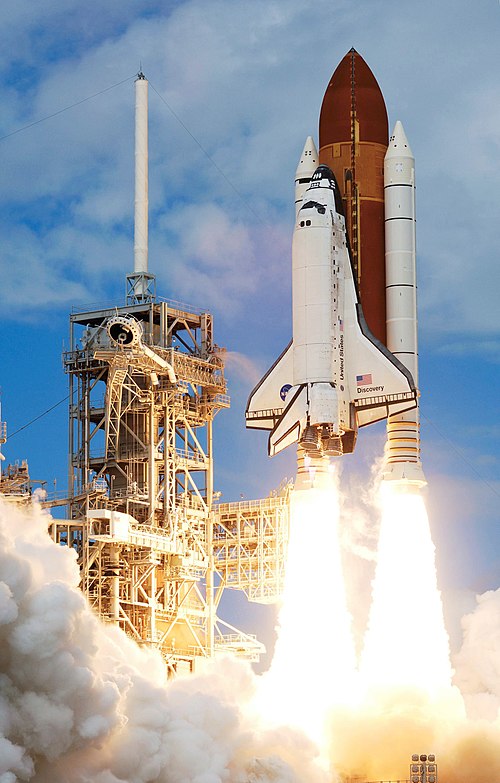
12 April 1981 marked a new era in manned spaceflight: Space Shuttle Columbia lifted off for the first time from Cape Canaveral. The Shuttle capped an incredible fruitful period in aerospace engineering development. The ground work laid by the original Wright flyer, the Spitfire, the X-1 and the X-15 is all part of the technological arc that led to the Shuttle. The fundamentals didn’t change but their orders of magnitude did.
“Like bolting a butterfly onto a bullet” — Story Musgrave, Columbia astronaut, 1996
Story Musgrave’s description of the Space Shuttle is not far off the mark. On the launch pad the Shuttle sat on two solid-rocket boosters producing 37 million horsepower, accelerating the Shuttle beyond the speed of sound in about 30 seconds. Eight minutes and 500,000 gallons of fuel later the Shuttle was travelling at 17,500 mph at the edge of space. The Space Shuttle was not only powerful but possessed a grace that the Wright brothers would have appreciated. After smashing through the atmosphere upon reentry at Mach 28 (8 km/s) the piloting astronaut had to slow the Shuttle down to 200 mph via a series of gliding twists and turns, using the surrounding air as an aerodynamic break.
The ultimate mission of the Shuttle was to serve as a cost-effective means of travelling to space for professional astronauts and civilians. That vision never came to fruition due to the high maintenance costs between flights, and partly due the Challenger and Columbia disasters that shattered all hopes that space travel would become routine.
Perhaps the Space Shuttle is one of humanities greatest inventions because it reminds us that for all its power, grace and genius it is still the brainchild of fallible men.
Edits:
A previous version of this article incorrectly stated that the Space Shuttle featured three solid rocket boosters (SRBs). Of course, the Space Shuttle only featured two.
At the start of the 19th century, after studying the highly cambered thin wings of many different birds, Sir George Cayley designed and built the first modern aerofoil, later used on a hand-launched glider. This biomimetic, highly cambered and thin-walled design remained the predominant aerofoil shape for almost 100 years, mainly due to the fact that the actual mechanisms of lift and drag were not understood scientifically but were explored in an empirical fashion. One of the major problems with these early aerofoil designs was that they experienced a phenomenon now known as boundary layer separation at very low angles of attack. This significantly limited the amount of lift that could be created by the wings and meant that bigger and bigger wings were needed to allow for any progress in terms of aircraft size. Lacking the analytical tools to study this problem, aerodynamicists continued to advocate thin aerofoil sections, as there was plenty of evidence in nature to suggest their efficacy. The problem was considered to be more one of degree, i.e. incrementally iterating the aerofoil shapes found in nature, rather than of type, that is designing an entirely new shape of aerofoil in accord with fundamental physics.
During the pre-WWI era, the misguided notions of designers was compounded by the ever-increasing use of wind-tunnel tests. The wind tunnels used at the time were relatively small and ran at very low flow speeds. This meant that the performance of the aerofoils was being tested under the conditions of laminar flow (smooth flow in layers, no mixing perpendicular to flow direction) rather than the turbulent flow (mixing of flow via small vortices) present over the wing surfaces. Under laminar flow conditions, increasing the thickness of an aerofoil increases the amount of skin-friction drag (as shown in last month’s post), and hence thinner aerofoils were considered to be superior.
The modern plane – born in 1915
The situation in Germany changed dramatically during WWI. In 1915 Hugo Junkers pioneered the first practical all-metal aircraft with a cantilevered wing – essentially the same semi-monocoque wing box design used today. The most popular design up to then was the biplane configuration held together by wires and struts, which introduced considerable amounts of parasitic drag and thereby limited the maximum speed of aircraft. Eliminating these supporting struts and wires meant that the flight loads needed to be carried by other means. Junkers cantilevered a beam from either side of the fuselage, the main spar, at about 25% of the chord of the wing to resist the up and down bending loads produced by lift. Then he fitted a smaller second spar, known as the trailing edge spar, at 75% of the chord to assist the main spar in resisting fore and aft bending induced by the drag on the wing. The two spars were connected by the external wing skin to produce a closed box-section known as the wing box. Finally, a curved piece of metal was fitted to the front of the wing to form the “D”-shaped leading edge, and two pieces of metal were run out to form the trailing edge. This series of three closed sections provided the wing with sufficient torsional rigidity to sustain the twisting loads that arise because the centre of pressure (the point where the lift force can be considered to act) is offset from the shear centre (the point where a vertical load will only cause bending and no twisting). Junker’s ideas were all combined in the world’s first practical all-metal aircraft, the Junker J 1, which although much heavier than other aircraft at the time, developed into the predominant form of construction for the larger and faster aircraft of the coming generation.
Junkers J 1 at Döberitz in 1915Structures + Aerodynamics = Superior Aircraft
Junkers construction naturally resulted in a much thicker wing due to the room required for internal bracing, and this design provided the impetus for novel aerodynamics research. Junker’s ideas were supported by Ludwig Prandtl who carried out his famous aerodynamics work at the University of Göttingen. As discussed in last month’s post, Prandtl had previously introduced the notion of the boundary layer; namely the existence of a U-shaped velocity profile with a no-flow condition at the surface and an increasing velocity field towards the main stream some distance away from the surface. Prandtl argued that the presence of a boundary layer supported the simplifying assumption that fluid flow can be split into two non-interacting portions; a thin layer close to the surface governed by viscosity (the stickiness of the fluid) and an inviscid mainstream. This allowed Prandtl and his colleagues to make much more accurate predictions of the lift and drag performance of specific wing-shapes and greatly helped in the design of German WWI aircraft. In 1917 Prandtl showed that Junker’s thick and less-cambered aerofoil section produced much more favourable lift characteristics than the classic thinner sections used by Germany’s enemies. Second, the thick aerofoil could be flown at a much higher angle of attack without stalling and hence improved the manoeuvrability of a plane during dog fighting.
Skin Friction versus Pressure Drag
The flow in a boundary layer can be either laminar or turbulent. Laminar flow is orderly and stratified without interchange of fluid particles between individual layers, whereas in turbulent flow there is significant exchange of fluid perpendicular to the flow direction. The type of flow greatly influences the physics of the boundary layer. For example, due to the greater extent of mass interchange, a turbulent boundary layer is thicker than a laminar one and also features a steeper velocity gradient close to the surface, i.e. the flow speed increases more quickly as we move away from the wall.
Velocity profile of laminar versus turbulent boundary layer. Note how the turbulent flow increases velocity more rapidly away from the wall.
Just like your hand experiences friction when sliding over a surface, so do layers of fluid in the boundary layer, i.e. the slower regions of the flow are holding back the faster regions. This means that the velocity gradient throughout the boundary layer gives rise to internal shear stresses that are akin to friction acting on a surface. This type of friction is aptly called skin-friction drag and is predominant in streamlined flows where the majority of the body’s surface is aligned with the flow. As the velocity gradient at the surface is greater for turbulent than laminar flow, a streamlined body experiences more drag when the boundary layer flow over its surfaces is turbulent. A typical example of a streamlined body is an aircraft wing at cruise, and hence it is no surprise that maintaining laminar flow over aircraft wings is an ongoing research topic.
Over flat surfaces we can suitably ignore any changes in pressure in the flow direction. Under these conditions, the boundary layer remains stable but grows in thickness in the flow direction. This is, of course, an idealised scenario and in real-world applications, such as curved wings, the flow is most likely experiencing an adverse pressure gradient, i.e. the pressure increases in the flow direction. Under these conditions the boundary layer can become unstable and separate from the surface. The boundary layer separation induces a second type of drag, known as pressure drag. This type of drag is predominant for non-streamlined bodies, e.g. a golfball flying through the air or an aircraft wing at a high angle of attack.
So why does the flow separate in the first place?
To answer this question consider fluid flow over a cylinder. Right at the front of the cylinder fluid particles must come to rest. This point is aptly called the stagnation point and is the point of maximum pressure (to conserve energy the pressure needs to fall as fluid velocity increases, and vice versa). Further downstream, the curvature of the cylinder causes the flow lines to curve, and in order to equilibrate the centripetal forces, the flow accelerates and the fluid pressure drops. Hence, an area of accelerating flow and falling pressure occurs between the stagnation point and the poles of the cylinder. Once the flow passes the poles, the curvature of the cylinder is less effective at directing the flow in curved streamlines due to all the open space downstream of the cylinder. Hence, the curvature in the flow reduces and the flow slows down, turning the previously favourable pressure gradient into an adverse pressure gradient of rising pressure.
Boundary layer separation over a cylinder (axis out out the page).
To understand boundary layer separation we need to understand how these favourable and adverse pressure gradients influence the shape of the boundary layer. From our discussion on boundary layers, we know that the fluid travels slower the closer we are to the surface due to the retarding action of the no-slip condition at the wall. In a favourable pressure gradient, the falling pressure along the streamlines helps to urge the fluid along, thereby overcoming some of the decelerating effects of the fluid’s viscosity. As a result, the fluid is not decelerated as much close to the wall leading to a fuller U-shaped velocity profile, and the boundary layer grows more slowly.
By analogy, the opposite occurs for an adverse pressure gradient, i.e. the mainstream pressure increases in the flow direction retarding the flow in the boundary layer. So in the case of an adverse pressure gradient the pressure forces reinforce the retarding viscous friction forces close to the surface. As a result, the difference between the flow velocity close to the wall and the mainstream is more pronounced and the boundary layer grows more quickly. If the adverse pressure gradient acts over a sufficiently extended distance, the deceleration in the flow will be sufficient to reverse the direction of flow in the boundary layer. Hence the boundary layer develops a point of inflection, known as the point of boundary layer separation, beyond which a circular flow pattern is established.
For aircraft wings, boundary layer separation can lead to very significant consequences ranging from an increase in pressure drag to a dramatic loss of lift, known as aerodynamic stall. The shape of an aircraft wing is essentially an elongated and perhaps asymmetric version of the cylinder shown above. Hence the airflow over the top convex surface of a wing follows the same basic principles outlined above:
There is a point of stagnation at the leading edge.
A region of accelerating mainstream flow (favourable pressure gradient) up to the point of maximum thickness.
A region of decelerating mainstream flow (adverse pressure gradient) beyond the point of maximum thickness.
These three points are summarised in the schematic diagram below.
Boundary layer separation over the top surface of a wing.
Boundary layer separation is an important issue for aircraft wings as it induces a large wake that completely changes the flow downstream of the point of separation. Skin-friction drag arises due to inherent viscosity of the fluid, i.e. the fluid sticks to the surface of the wing and the associated frictional shear stress exerts a drag force. When a boundary layer separates, a drag force is induced as a result of differences in pressure upstream and downstream of the wing. The overall dimensions of the wake, and therefore the magnitude of pressure drag, depends on the point of separation along the wing. The velocity profiles of turbulent and laminar boundary layers (see image above) show that the velocity of the fluid increases much slower away from the wall for a laminar boundary layer. As a result, the flow in a laminar boundary layer will reverse direction much earlier in the presence of an adverse pressure gradient than the flow in a turbulent boundary layer.
To summarise, we now know that the inherent viscosity of a fluid leads to the presence of a boundary layer that has two possible sources of drag. Skin-friction drag due to the frictional shear stress between the fluid and the surface, and pressure drag due to flow separation and the existence of a downstream wake. As the total drag is the sum of these two effects, the aerodynamicist is faced with a non-trivial compromise:
skin-friction drag is reduced by laminar flow due to a lower shear stress at the wall, but this increases pressure drag when boundary layer separation occurs.
pressure drag is reduced by turbulent flow by delaying boundary layer separation, but this increases the skin-friction drag due to higher shear stresses at the wall.
As a result, neither laminar nor turbulent flow can be said to be preferable in general and judgement has to be made regarding the specific application. For a blunt body, such as a cylinder, pressure drag dominates and therefore a turbulent boundary layer is preferable. For more streamlined bodies, such as an aircraft wing at cruise, the overall drag is dominated by skin-friction drag and hence a laminar boundary layer is preferable. Dolphins, for example, have very streamlined bodies to maintain laminar flow. Early golfers, on the other hand, realised that worn rubber golf balls flew further than pristine ones, and this led to the innovation of dimples on golf balls. Fluid flow over golf balls is predominantly laminar due to the relatively low flight speeds. Dimples are therefore nothing more than small imperfections that transform the predominantly laminar flow into a turbulent one that delays the onset of boundary layer separation and therefore reduces pressure drag.
Aerodynamic Stall
The second, and more dramatic effect, of boundary layer separation in aircraft wings is aerodynamic stall. At relatively low angles of attack, for example during cruise, the adverse pressure gradient acting on the top surface of the wing is benign and the boundary layer remains attached over the entire surface. As the angle of attack is increased, however, so does the pressure gradient. At some point the boundary layer will start to separate near the trailing edge of the wing, and this separation point will move further upstream as the angle of attack is increased. If an aerofoil is positioned at a sufficiently large angle of attack, separation will occur very close to the point of maximum thickness of the aerofoil and a large wake will develop behind the point of separation. This wake redistributes the flow over the rest of the aerofoil and thereby significantly impairs the lift generated by the wing. As a result, the lift produced is seriously reduced in a condition known as aerodynamic stall. Due to the high pressure drag induced by the wake, the aircraft can further lose airspeed, pushing the separation point further upstream and creating a deleterious feedback loop where the aircraft literally starts to fall out of the sky in an uncontrolled spiral. To prevent total loss of control, the pilot needs to reattach the boundary as quickly as possible which is achieved by reducing the angle of attack and pointing the nose of the aircraft down to gain speed.
The lift produced by a wing is given by
[latex]L = \frac{1}{2}C_L \rho V^2 S[/latex]
where [latex]\rho[/latex] is the density of the surrounding air, [latex]V[/latex] is the flight velocity, [latex]S[/latex] is the wing area and [latex]C_L[/latex] is the lift coefficient of the aerofoil shape. The lift coefficient of a specific aerofoil shape increases linearly with the angle of attack up to a maximum point [latex]C_{Lmax}[/latex]. The maximum lift coefficient of a typical aerofoil is around 1.4 at an angle of attack of around [latex]16^\circ[/latex], which is bounded by the critical angle of attack where the stall condition occurs.
During cruise the angle of attack is relatively small ([latex]\approx 2^\circ[/latex]) as sufficient lift is guaranteed by the high flight velocity [latex]V[/latex]. Furthermore, we actually want to maintain a small angle of attack as this minimises the pressure drag induced by boundary layer separation. At takeoff and landing, however, the flight velocity is much smaller which means that the lift coefficient has to be increased by setting the wings at a more aggressive angle of attack ([latex]\approx 15^\circ[/latex]). The issue is that even with a near maximum lift coefficient of 1.4, large jumbo jets have a hard time achieving the necessary lift force at safe speeds for landing. While it would also be possible to increase the wing area, such a solution would have detrimental effect on the aircraft weight and therefore fuel efficiency.
High-lift Devices
A much more elegant solution are leading-edge slats and trailing-edge flaps. A slat is a thin, curved aerofoil that is fitted to the front of the wing and is intended to induce a secondary airflow through the gap between the slat and the leading edge. The air accelerates through this gap and thereby injects high momentum fluid into the boundary on the upper surface, delaying the onset of flow reversal in the boundary layer. Similarly, one or two curved aerofoils may be placed at the rear of wing in order to invigorate the flow near the trailing edge. In this case the high momentum fluid reinvigorates the flow which has been slowed down by the adverse pressure gradient. The maximum lift coefficient can typically be doubled by these devices and therefore allows big jumbo jets to land and takeoff at relatively low runway speeds.
Leading edge slats and trailing edge flaps on an aircraft wing
The next time you are sitting close to the wings observe how these devices are retracted after take-off and activated before landing. In fact, birds have a similar devices on their wings. The wings of bats are comprised of thin and flexible membranes reinforced by small bones which roughen the membrane surface and help to transition the flow from laminar to turbulent and prevent boundary layer separation. As is so often the case in engineering design, a lot of inspiration can be taken from nature!
In the early 20th century, a group of German scientists led by Ludwig Prandtl at the University of Göttingen began studying the fundamental nature of fluid flow and subsequently laid the foundations for modern aerodynamics. In 1904, just a year after the first flight by the Wright brothers, Prandtl published the first paper on a new concept, now known as the boundary layer. In the following years, Prandtl worked on supersonic flow and spent most of his time developing the foundations for wing theory, ultimately leading to the famous red triplane flown by Baron von Richthofen, the Red Baron, during WWI.
Prandtl’s key insight in the development of the boundary layer was that as a first-order approximation it is valid to separate any flow over a surface into two regions: a thin boundary layer near the surface where the effects of viscosity cannot be ignored, and a region outside the boundary layer where viscosity is negligible. The nature of the boundary layer that forms close to the surface of a body significantly influences how the fluid and body interact. Hence, an understanding of boundary layers is essential in predicting how much drag an aircraft experiences, and is therefore a mandatory requirement in any first course on aerodynamics.
Boundary layers develop due to the inherent stickiness or viscosity of the fluid. As a fluid flows over a surface, the fluid sticks to the solid boundary which is the so-called “no-slip condition”. As sudden jumps in flow velocity are not possible for flow continuity requirements, there must exist a small region within the fluid, close to the body over which the fluid is flowing, where the flow velocity increases from zero to the mainstream velocity. This region is the so-called boundary layer.
The U-shaped profile of the boundary layer can be visualised by suspending a straight line of dye in water and allowing fluid flow to distort the line of dye (see below). The distance of a distorted dye particle to its original position is proportional to the flow velocity. The fluid is stationary at the wall, increases in velocity moving away from the wall, and then converges to the constant mainstream value [latex]u_0[/latex] at a distance [latex]\delta[/latex] equal to the thickness of the boundary layer.
To further investigate the nature of the flow within the boundary layer, let’s split the boundary layer into small regions parallel to the surface and assume a constant fluid velocity within each of these regions (essentially the arrows in the figure above). We have established that the boundary layer is driven by viscosity. Therefore, adjacent regions within the boundary layer that move at slightly different velocities must exert a frictional force on each other. This is analogous to you running your hand over a table-top surface and feeling a frictional force on the palm of your hand. The shear stresses [latex]\tau[/latex] inside the fluid are a function of the viscosity or stickiness of the fluid [latex]\mu[/latex], and also the velocity gradient [latex]du/dy[/latex]:
where [latex]y[/latex] is the coordinate measuring the distance from the solid boundary, also called the “wall”.
Prandtl first noted that shearing forces are negligible in mainstream flow due to the low viscosity of most fluids and the near uniformity of flow velocities in the mainstream. In the boundary layer, however, appreciable shear stresses driven by steep velocity gradients will arise.
So the pertinent question is: Do these two regions influence each other or can they be analysed separately?
Prandtl argued that for flow around streamlined bodies, the thickness of the boundary layer is an order of magnitude smaller than the thickness of the mainstream, and therefore the pressure and velocity fields around a streamlined body may analysed disregarding the presence of the boundary layer.
Eliminating the effect of viscosity in the free flow is an enormously helpful simplification in analysing the flow. Prandtl’s assumption allows us to model the mainstream flow using Bernoulli’s equation or the equations of compressible flow that we have discussed before, and this was a major impetus in the rapid development of aerodynamics in the 20th century. Today, the engineer has a suite of advanced computational tools at hand to model the viscid nature of the entire flow. However, the idea of partitioning the flow into an inviscid mainstream and viscid boundary layer is still essential for fundamental insights into basic aerodynamics.
Laminar and turbulent boundary layers
One simple example that nicely demonstrates the physics of boundary layers is the problem of flow over a flat plate.
Development of boundary layer over a flat plate including the transition from a laminar to turbulent boundary layer.
The fluid is streaming in from the left with a free stream velocity [latex]U_0[/latex] and due to the no-slip condition slows down close to the surface of the plate. Hence, a boundary layer starts to form at the leading edge. As the fluid proceeds further downstream, large shearing stresses and velocity gradients develop within the boundary layer. Proceeding further downstream, more and more fluid is slowed down and therefore the thickness, [latex]\delta[/latex], of the boundary layer grows. As there is no sharp line splitting the boundary layer from the free-stream, the assumption is typically made that the boundary layer extends to the point where the fluid velocity reaches 99% of the free stream. At all times, and at at any distance [latex]x[/latex] from the leading edge, the thickness of the boundary layer [latex]\delta[/latex] is small compared to [latex]x[/latex].
Close to the leading edge the flow is entirely laminar, meaning the fluid can be imagined to travel in strata, or lamina, that do not mix. In essence, layers of fluid slide over each other without any interchange of fluid particles between adjacent layers. The flow speed within each imaginary lamina is constant and increases with the distance from the surface. The shear stress within the fluid is therefore entirely a function of the viscosity and the velocity gradients.
Further downstream, the laminar flow becomes unstable and fluid particles start to move perpendicular to the surface as well as parallel to it. Therefore, the previously stratified flow starts to mix up and fluid particles are exchanged between adjacent layers. Due to this seemingly random motion this type of flow is known as turbulent. In a turbulent boundary layer, the thickness [latex]\delta[/latex] increases at a faster rate because of the greater extent of mixing within the main flow. The transverse mixing of the fluid and exchange of momentum between individual layers induces extra shearing forces known as the Reynolds stresses. However, the random irregularities and mixing in turbulent flow cannot occur in the close vicinity of the surface, and therefore a viscous sublayer forms beneath the turbulent boundary layer in which the flow is laminar.
An excellent example contrasting the differences in turbulent and laminar flow is the smoke rising from a cigarette.
Laminar and turbulent flow in smoke
As smoke rises it transforms from a region of smooth laminar flow to a region of unsteady turbulent flow. The nature of the flow, laminar or turbulent, is captured very efficiently in a single parameter known as the Reynolds number
[latex]Re = \frac{\rho U d}{\mu}[/latex]
where [latex]\rho[/latex] is the density of the fluid, [latex]U[/latex] the local flow velocity, [latex]d[/latex] a characteristic length describing the geometry, and [latex]\mu[/latex] is the viscosity of the fluid.
There exists a critical Reynolds number in the region [latex]2300-4000[/latex] for which the flow transitions from laminar to turbulent. For the plate example above, the characteristic length is the distance from the leading edge. Therefore [latex]d[/latex] increases as we proceed downstream, increasing the Reynolds number until at some point the flow transitions from laminar to turbulent. The faster the free stream velocity [latex]U[/latex], the shorter the distance from the leading edge where this transition occurs.
Velocity profiles
Due to the different degrees of fluid mixing in laminar and turbulent flows, the shape of the two boundary layers is different. The increase in fluid velocity moving away from the surface (y-direction) must be continuous in order to guarantee a unique value of the velocity gradient [latex]du/dy[/latex]. For a discontinuous change in velocity, the velocity gradient [latex]du/dy[/latex], and therefore the shearing forces [latex] \tau = \mu \frac{\mathrm{d}u}{\mathrm{d}y}[/latex] would be infinite, which is obviously not feasible in reality. Hence, the velocity increases smoothly from zero at the wall in some form of parabolic distribution. The further we move away from the wall, the smaller the velocity gradient and the retarding action of the shearing stresses decreases.
In the case of laminar flow, the shape of the boundary layer is indeed quite smooth and does not change much over time. For a turbulent boundary layer however, only the average shape of the boundary layer approximates the parabolic profile discussed above. The figure below compares a typical laminar layer with an averaged turbulent layer.
Velocity profile of laminar versus turbulent boundary layer
In the laminar layer, the kinetic energy of the free flowing fluid is transmitted to the slower moving fluid near the surface purely means by of viscosity, i.e. frictional shear stresses. Hence, an imaginary fluid layer close to the free stream pulls along an adjacent layer close to the wall, and so on. As a result, significant portions of fluid in the laminar boundary layer travel at a reduced velocity. In a turbulent boundary layer, the kinetic energy of the free stream is also transmitted via Reynolds stresses, i.e. momentum exchanges due to the intermingling of fluid particles. This leads to a more rapid rise of the velocity away from the wall and a more uniform fluid velocity throughout the entire boundary layer. Due to the presence of the viscous sublayer in the close vicinity of the wall, the wall shear stress in a turbulent boundary layer is governed by the usual equation [latex] \tau = \mu \frac{\mathrm{d}u}{\mathrm{d}y}[/latex]. This means that because of the greater velocity gradient at the wall the frictional shear stress in a turbulent boundary is greater than in a purely laminar boundary layer.
Skin Friction drag
Fluids can only exert two types of forces: normal forces due to pressure and tangential forces due to shear stress. Pressure drag is the phenomenon that occurs when a body is oriented perpendicular to the direction of fluid flow. Skin friction drag is the frictional shear force exerted on a body aligned parallel to the flow, and therefore a direct result of the viscous boundary layer.
Due to the greater shear stress at the wall, the skin friction drag is greater for turbulent boundary layers than for laminar ones. Skin friction drag is predominant in streamlined aerodynamic profiles, e.g. fish, airplane wings, or any other shape where most of the surface area is aligned with the flow direction. For these profiles, maintaining a laminar boundary layer is preferable. For example, the crescent lunar shaped tail of many sea mammals or fish has evolved to maintain a relatively constant laminar boundary layer when oscillating the tail from side to side.
One of Prandtl’s PhD students, Paul Blasius, developed an analytical expression for the shape of a laminar boundary layer over a flat plate without a pressure gradient. Blasius’ expression has been verified by experiments many times over and is considered a standard in fluid dynamics. The two important quantities that are of interest to the designer are the boundary layer thickness [latex]\delta[/latex] and the shear stress at the wall [latex]\tau_w[/latex] at a distance [latex]x[/latex] from the leading edge. The boundary layer thickness is given by
[latex] \delta=\frac{5.2 x}{\sqrt{Re_x}}[/latex]
with [latex]Re_x[/latex] the Reynolds number at a distance [latex]x[/latex] from the leading edge. Due to the presence of [latex]x[/latex] in the numerator and [latex]\sqrt{x}[/latex] in the denominator, the boundary layer thickness scales proportional to [latex]x^{1/2}[/latex], and hence increases rapidly in the beginning before settling down.
Next, we can use a similar expression to determine the shear stress at the wall. To do this we first define another non dimensional number known as the drag coefficient
[latex]C_f=\frac{\tau_w}{1/2 \rho U_f^2}[/latex]
which is the value of the shear stress at the wall normalised by the dynamic pressure of the free-flow. According to Blasius, the skin-friction drag coefficient is simply governed by the Reynolds number
[latex]C_f=\frac{0.664}{\sqrt{Re_x}}[/latex]
This simple example reiterates the power of dimensionless numbers we mentioned before when discussing wind tunnel testing. Even though the shear stress at the wall is a dimensional quantity, we have been able to express it merely as a function of two non-dimensional quantities [latex]Re[/latex] and [latex]C_f[/latex]. By combining the two equations above, the shear stress can be written as
and therefore scales proportional to [latex]x^{-1/2}[/latex], tending to zero as the distance from the leading edge increases. The value of [latex]\tau_w[/latex] is the frictional shear stress at a specific point [latex]x[/latex] from the leading edge. To find the total amount of drag [latex]D_{sf}[/latex] exerted on the plate we need to sum up (integrate) all contributions of [latex]\tau_w[/latex] over the length of the plate
where [latex]Re_L[/latex] is now the Reynolds number of the free stream calculated using the total length of the plate [latex]L[/latex]. Similar to the skin friction coefficient [latex]C_f[/latex] we can define a total skin friction drag coefficient [latex]\eta_f[/latex]
Hence, [latex]C_f[/latex] can be used to calculate the local amount of shear stress at a point [latex]x[/latex] from the leading edge, whereas [latex]\eta_f[/latex] is used to find the total amount of skin friction drag acting on the surface.
Unfortunately, do to the chaotic nature of turbulent flow, the boundary layer thickness and skin drag coefficient for a turbulent boundary layer cannot be determined as easily in a theoretical manner. Therefore we have to rely on experimental results to define empirical approximations of these quantities. The scientific consensus of the these relations are as follows:
Therefore the thickness of a turbulent boundary layer grows proportional to [latex]x^{4/5}[/latex] (faster than the [latex]x^{1/2}[/latex] relation for laminar flow) and the total skin friction drag coefficient varies as [latex]L^{-1/5}[/latex] (also faster than the [latex]L^{-1/2}[/latex] relation of laminar flow). Hence, the total skin drag coefficient confirms the qualitative observations we made before that the frictional shear stresses in a turbulent boundary layer are greater than those in a laminar one.
Skin friction drag and wing design
The unfortunate fact for aircraft designers is that turbulent flow is much more common in nature than laminar flow. The tendency for flow to be random rather than layered can be interpreted in a similar way to the second law of thermodynamics. The fact that entropy in a closed system only increases is to say that, if left to its own devices, the state in the system will tend from order to disorder. And so it is with fluid flow.
However, the shape of a wing can be designed in such a manner as to encourage the formation of laminar flow. The P-51 Mustang WWII fighter was the first production aircraft designed to operate with laminar flow over its wings. The problem back then, and to this day, is that laminar flow is incredibly unstable. Protruding rivet heads or splattered insects on the wing surface can easily “trip” a laminar boundary layer into turbulence, and preempt any clever design the engineer concocted. As a result, most of the laminar flow wings that have been designed based on idealised conditions and smooth wing surfaces in a wind tunnel have not led to the sweeping improvements originally imagined.
For many years NASA conducted a series of experiments to design a natural laminar flow (NLF) aircraft. Some of their research suggested the wrapping of a glove around the leading edge of a Boeing 757 just outboard of the engine. The modified shape of this wing promotes laminar flow at the high altitudes and almost sonic flight conditions of a typical jet airliner. To prevent the build up of insect splatter at take-off a sheath of paper was wrapped around the glove which was then torn away at altitude. Even though the range of such an aircraft could be increased by almost 15% this, rather elaborate scheme, never made it into production.
In the mid 1990s NASA fitted active test panels to the wings of two F-16’s in order to test the possibility of achieving laminar flow on swept delta-wings flying at supersonic speed; in NASA’s view a likely wing configuration for future supersonic cruise aircraft. The active test panels essentially consisted of titanium covers perforated with millions of microscopic holes, which were attached to the leading edge and the top surface of the wing. The role of these panels was to suck most of the boundary layer off the top surface through perforations using an internal pumping system. By removing air from the boundary layer its thickness decreased and thereby promoted the stability of the laminar boundary layer over the wing. This Supersonic Laminar Flow (SLFC) project successfully maintained laminar flow over a large portion of the wing during supersonic flight of up to Mach 1.6.
F-16 XL with suction panels to promote laminar flow
While these elaborate schemes have not quite found their way into mass production (probably due to their cost, maintenance problems and risk), laminar flow wings are a very viable future technology in terms of reducing greenhouse gases as stipulated by environmental legislation. An important driver in reducing greenhouse gases is maximising the lift-to-drag ratio of the wings, and therefore I would expect research to continue in this field for some time to come.
Despite the growing computer power and increasing sophistication of computational models, any design meant operate in the real world requires some form of experimental validation. The idealist modeller, me included, wants to believe that computer simulation will replace all forms of experimental testing and thereby allow for much faster design cycles. The issue with this is that random imperfections, and most importantly their concurrence, are very hard to account for robustly, especially when operating in nonlinear domains. As a result, the quantity and quality of both computational and experimental validation have increased in lockstep over the few last decades.
In “The Wind and Beyond”, the autobiography of Theodore von Kármán, one of the pre-eminent aerospace engineers and scientists of the 20th century, von Kármán recounts a telling episode regarding the role of wind tunnel testing in the development of the Douglas DC-3, the first American commercial jetliner. Early versions of the DC-3 faced a problem with aerodynamic instabilities that could throw the airplane out of control. A similar problem had been noticed earlier on the Northrop Alpha airplane, which, like the DC-3, featured a wing that was attached to the underside of the fuselage. When two of von Kármán’s assistants, Major Klein and Clark Millikan, subjected a model of the Alpha to high winds in a wind tunnel, the model aircraft started to sway and shake violently. In the following investigation, Klein and Millikan found that the sharp corner at the connection between the wing and fuselage decelerated the air as it flowed past, causing boundary layer separation and a wake of eddies. As these eddies broke away from the trailing edge of the wing, they adversely impacted the flow over the horizontal stabiliser and vertical tail fin at the rear of the aircraft and resulted in uncontrollable vibrations.
The Northrop Alpha plane with the Kármán fillet at the wing-fuselage jointFortunately, Theodore von Kármán was world-renowned, among other things, for his work on eddies and especially the so-called von Kármán Vortex Street. Von Kármán therefore intuitively realised what had to be done to eliminate the creation of these eddies. Von Kármán and his colleagues fitted a small fairing, a filling if you like, to the connection between the wing and the fuselage to smooth out the eddies. This became one of the textbook examples of how wind tunnel findings could be applied in a practical way to iron out problems with an aircraft. When French engineers learned of the device from von Kármán at a conference a few years later, they were so enamoured that such a simple idea could solve such a big problem that they named the fillet a “Kármán”.
When testing the aerodynamics of aircraft, the wind tunnel is indispensable. The Wright brothers built their own wind tunnel to validate the research data on airfoils that had been recorded throughout the 19th century. One of the most important pieces of equipment in the early days of NACA (now NASA) was a variable-density wind tunnel, which by pressurising the air, allowed realistic operating conditions to be simulated on 1/20th geometrically-scaled models.
NACA variable density wind tunnelThis brings us to an important point: How do you test the aerodynamics of an aircraft in a wind-tunnel?
Do you need to build individual wind-tunnels big enough to fit a particular aircraft? Or can you use a smaller multi-purpose wind tunnel to test small-scale models of the actual aircraft? If this is the case, how representative is the collected data of the actual flying aircraft?
Luckily we can make use of some clever mathematics, known as dimensional analysis, to make our life a little easier. The key idea behind dimensional analysis is to define a set of dimensionless parameters that govern the physical behaviour of the phenomenon being studied, purely by identifying the fundamental dimensions (time, length and mass in aerodynamics) that are at play. This is best illustrated by an example.
The United States developed the atomic bomb during WWII under the greatest security precautions. Even many years after the first test of 1945 in the desert of New Mexico, the total amount of energy released during the explosion remained unknown. The British scientist G.I. Taylor then famously estimated the total amount of energy released by the explosion simply by using available pictures showing the explosion plume at different time stamps after detonation.
Nuclear explosion time frames
By assuming that the shock wave could be modelled as a perfect sphere, Taylor posited that the size of the plume, i.e. the radius [latex]R[/latex], should depend on the energy [latex]E[/latex] of the explosion, the time [latex]t[/latex] after detonation and the density [latex]\rho[/latex] of the surrounding air.
In dimensional analysis we proceed to define the fundamental units or dimensions that quantify our variables. So in this case:
Radius is defined by a distance, and therefore the units are length, i.e. [latex][R] = L.[/latex]
The units of time are, you guessed it, time, i.e. [latex][t] = T.[/latex]
Energy is force times distance, where a force is mass times acceleration, and acceleration is distance divided by time squared i.e. [latex][E] = \left(\frac{ML}{T^2}\right)L = \frac{M L^2}{T^2}.[/latex]
Density is mass divided by volume, where volume is a distance cubed, i.e. [latex][\rho] = \frac{M}{L^3}.[/latex]
Having determined all our variables in the fundamental dimensions of distance, time and mass, we now attempt to relate the radius of the explosion to the energy, density and time. If we assume that the radius is proportional to these three variables, then dividing the radius by the product of the other three variables must result in a dimensionless number. Hence,
[latex]c = \frac{R}{E^x \rho^y t^z}[/latex]
Or alternatively, all fundamental dimensions in the above fraction must cancel:
For all units to disappear we need:
[latex]-x-y = 0 \qquad 1-2x+3y=0 \qquad 2x – z =0[/latex]
and solving this system gives:
[latex]x = 1/5 \qquad y = -1/5 \qquad z = 2/5 [/latex]
Therefore the shock wave radius is given by
[latex]R = c E^{1/5} \rho^{-1/5} t^{2/5} [/latex]
and by re-arranging
[latex]E = k \frac{R^5 \rho}{t^2}[/latex]
where [latex]k = \frac{1}{c^5}[/latex].
So, we have an expression that relates the energy of the explosion to the radius, the density of air and time after detonation, which were all available to Taylor from the individual time stamps (these provided a diameter estimate and the time after detonation. The density of the air was known).
In the example above, specific calculations of [latex]E[/latex] also require an estimate of the constant [latex]k[/latex]. In aerodynamics, we are typically interested in quantifying the constant itself using the variables at hand. Hence, by analogy with the above example, we would know the energy, the density, radius and time and then calculate a value for the constant under these conditions. As the constant is dimensionless, it allows us to make an unbiased judgement of the flow conditions for entirely different and unrelated problems.
The most famous dimensionless number in aerodynamics is probably the Reynolds number which quantifies the nature of the flow, i.e. is it laminar (nice and orderly in layers that do not mix), or is it turbulent, or somewhere in between?
In determining aerodynamic forces, two of the important variables we want to understand and quantify are the lift and drag. Particularly, we want to determine how the lift and drag vary with independent parameters such as the flight velocity, wing area and the properties of the surrounding area.
Using a similar method as above, it can be shown that the two primary dimensionless variables are the lift ([latex]C_L[/latex]) and drag coefficients ([latex]C_D[/latex]), which are defined in terms of lift ([latex]L[/latex]), drag ([latex]D[/latex]), flight velocity ([latex]U[/latex]), static fluid density ([latex]\rho[/latex]) and wing area ([latex]S[/latex]).
Lift coefficient:
[latex]C_L = \frac{L}{1/2 \rho U^2 S}[/latex]
Drag coefficient:
[latex]C_D = \frac{D}{1/2 \rho U^2 S}[/latex]
where [latex]1/2 \rho U^2[/latex] is known as the dynamic pressure of a fluid in motion. When the dynamic pressure is multiplied by the wing area, [latex]S[/latex], we are left with units of force which cancel the unit of lift ([latex]L[/latex]) and drag ([latex]D[/latex]), thus making [latex]C_L[/latex] and [latex]C_D[/latex] dimensionless.
As long as the geometry of our vehicle remains the same (scaling up and down at constant ratio of relative dimensions, e.g. length, width, height, wing span, chord etc.), these two parameters are only dependent on two other dimensionless variables: the Reynolds number
[latex]Re = \frac{\rho U c}{\mu}[/latex]
where [latex]U[/latex] and [latex]c[/latex] are characteristic flow velocity and length (usually aerofoil chord or wingspan), and the the Mach Number
[latex]M = \frac{U}{U_{sound}} = \frac{U}{\sqrt{\gamma R T}}[/latex]
which is the ratio of aircraft speed to the local speed of sound.
Let’s recap what we have developed until now. We have two dimensionless parameters, the lift and drag coefficients, which measure the amount of lift and drag an airfoil or flight vehicle creates normalised by the conditions of the surrounding fluid ([latex]1/2 \rho U^2[/latex]) and the geometry of the lifting surface ([latex]S[/latex]). Hence, these dimensionless parameters allow us to make a fair comparison of the performance of different airfoils regardless of their size. Comparing the [latex]C_L[/latex] and [latex]C_D[/latex] of two different airfoils requires that the operating conditions be comparable. They do not have to be exactly the same in terms of air speed, density and temperature but their dimensionless quantities, namely the Mach number and Reynolds number, need to be equal.
As an example consider a prototype aircraft flying at altitude and a scaled version of the same aircraft in a wind tunnel. The model and prototype aircraft have the same geometrical shape and only vary in terms of their absolute dimensions and the operating conditions. If the values of Reynolds number and Mach number of the flow are the same for both, then the flows are called dynamically similar, and as the geometry of the two aircraft are scaled version of each other, it follows that the lift and drag coefficients must be the same too. This concept of dynamic similarity is crucial for wind-tunnel experiments as it allows engineers to create small-scale models of full-sized aircraft and reliably predict their aerodynamic qualities in a wind tunnel.
This of course means that the wind tunnel needs to be operated at entirely different temperatures and pressures than the operating conditions at altitude. As long as the dimensions of the model remain in proportion upon scaling up or down, the model wing area scales with the square of the wing chord, i.e. [latex]S[/latex] is proportional to [latex]c^2[/latex]. We know from the explanation above that for a certain combination of Mach number and Reynolds number the lift and drag coefficients are fixed.
Using the definition of [latex]C_L[/latex] and [latex]C_D[/latex] the lift is given by
[latex]L = C_L * (1/2 \rho U^2 S)[/latex]
and the drag by
[latex]D = C_D * (1/2 \rho U^2 S)[/latex]
The lift and drag created by an aircraft or model under constant Mach number and Reynolds number scale with the wing area or the wing chord squared. Rearranging the equation for the Reynolds number, the wing chord can in fact be shown to be proportional to the operating temperature and pressure of the fluid flow. So by rearranging the Reynolds number equation:
[latex]Re = \frac{\rho U c}{\mu} \Rightarrow c = \frac{Re \mu}{\rho U}[/latex]
and from the fundamental gas equation
[latex]\rho = \frac{P}{RT}[/latex]
and the Mach Number we have
[latex]U = M \sqrt{\gamma RT}[/latex]
such that we can reformulate the chord length as follows
[latex]c = \frac{Re \mu RT}{P M \sqrt{\gamma RT}} = \frac{Re \mu \sqrt{RT}}{P M \sqrt{\gamma}}[/latex]
Hence, the chord of the model is inversely proportional to the fluid pressure and directly proportional to the square of the fluid temperature. Thus, maximising the pressure and reducing the temperature (maximum fluid density) reduces the required size of the model and the overall aerodynamic forces. The was the concept behind NACA’s early variable density tunnel and is still exploited in modern cryogenic wind tunnels.
This is the fourth and final part of a series of posts on rocket science. Part I covered the history of rocketry, Part II dealt with the operating principles of rockets and Part III looked at the components that go into the propulsive system.
One of the most important drivers in rocket design is the mass ratio, i.e. the ratio of fuel mass to dry mass of the rocket. The greater the mass ratio the greater the change in velocity (delta-v) the rocket can achieve. You can think of delta-v as the pseudo-currency of rocket science. Manoeuvres into orbit, to the moon or any other point in space are measured by their respective delta-v’s and this in turn defines the required mass ratio of the rocket.
For example, at an altitude of 200 km an object needs to travel at 7.8 km/s to inject into low earth orbit (LEO). Accounting for frictional losses and gravity, the actual requirement rocket scientists need to design for when starting from rest on a launch pad is just shy of delta-v=10 km/s. Using Tsiolovsky’s rocket equation and assuming a representative average exhaust velocity of 3500 m/s, this translates into a mass ratio of 17.4:
A mass ratio of 17.4 means that the rocket needs to be % fuel!
This simple example explains why the mass ratio is a key indicator of a rocket’s structural efficiency. The higher the mass ratio the greater the ratio of delta-v producing propellant to non-delta-v producing structural mass. The simple example also explains why staging is such an effective strategy. Once, a certain amount of fuel within the tanks has been used up, it is beneficial to shed the unnecessary structural mass that was previously used to contain the fuel but is no longer contributing to delta-v.
At the same time we need to ask ourselves how to best minimise the mass of the rocket structure?
So in this post we will turn to my favourite topic of all: Structural design. Let’s dig in…
The role of the rocket structure is to provide some form of load-bearing frame while simultaneously serving as an aerodynamic profile and container for propellant and payload. In order to maximise the mass ratio, the rocket designer wants to minimise the structural mass that is required to safely contain the propellant. There are essentially two ways to achieve this:
Using lightweight materials.
And/or optimising the geometric design of the structure.
When referring to “lightweight materials” what we mean is that the material has high values of specific stiffness, specific strength and/or specific toughness. In this case “specific” means that the classical engineering properties of elastic modulus (stiffness), yield or ultimate strength, and fracture toughness are weighted by the density of the material. For example, if a design of given dimensions (fixed volume) requires a certain stiffness and strength, and we can achieve these specifications with a material of superior specific properties, then the mass of the structure will be reduced compared to some other material. In the rocket industry the typical materials are aerospace-grade titanium and aluminium alloys as their specific properties are much more favourable than those of other metal alloys such as steel.
However, over the last 30 years there has been a drive towards increasing the proportion of advanced fibre-reinforced plastics in rocket structures. One of the issues with composites is that the polymer matrices that bind the fibres together become rather brittle (think of shattering glass) under the cryogenic temperatures of outer space or when in contact with liquid propellants. The second issue with traditional composites is that they are more flammable; obviously not a good thing when sitting right next to liquid hydrogen and oxygen. Third, it is harder to seal composite rocket tanks and especially bolted joints are prone to leaking. Finally, the high-performance characteristics that are needed for space applications require the use of massive high-pressure, high-temperature ovens (autoclaves) and tight-tolerance moulds which significantly drive up manufacturing costs. For these reasons the use composites is mostly restricted to payload fairings. NASA is currently working hard on their out-of-autoclave technology and automated fibre placement technology, while Rocket Lab already uses carbon-composite rockets.
The load-bearing structure in a rocket is very similar to the fuselage of an airplane and is based on the same design philosophy: semi-monocoque construction. In contrast to early aircraft that used frames of discrete members braced by wires to sustain flight loads and flexible membranes as lift surfaces, the major advantage of semi-monocoque construction is that the functions of aerodynamic profile and load-carrying structure are combined. Hence, the visible cylindrical barrel of a rocket serves to contain the internal fuel as a pressure vessel, sustains the imposed flights loads and also defines the aerodynamic shape of the rocket. Because the external skin is a working part of the structure, this type of construction is known as stressed skin or monocoque. The even distribution of material in a monocoque means that the entire structure is at a more uniform and lower stress state with fewer local stress concentrations that can be hot spots for crack initiation.
Second, curved shell structures, as in a cylindrical rocket barrel, are one of the most efficient forms of construction found in nature, e.g. eggs, sea-shells, nut-shells etc. In thin-walled curved structures the external loads are reacted internally by a combination of membrane stresses (uniform stretching or compression through the thickness) and bending stresses (linear variation of stresses through the thickness with tension on one side, compression on the other side, zero stress somewhere in the interior of the thickness known as the neutral axis). As a rule of thumb, membrane stresses are more efficient than bending stresses, as all of the material through the thickness is contributing to reacting the external load (no neutral axis) and the stress state is uniform (no stress concentrations).
In general, flat structures such as your typical credit card, will resist tensile and compressive external loads via uniform membrane stresses, and bending via linearly varying stresses through the thickness. The efficiency of curved shells stems from the fact that membrane stresses are induced to react both uniform stretching/compressive forces and bending moments. The presence of a membrane component reduces the peak stress that occurs through the thickness of the shell, and ultimately means that a thinner wall thickness and associated lower component mass will safely resist the externally applied loads. This is important as the bending stiffness of thin-walled structures is typically at least an order of magnitude smaller than the stretching/compressive stiffness (e.g. you can easily bend your credit card, but try stretching it).
Alas, as so often in life, there is a compromise. Optimising a structure for one mode of deformation typically makes it more fragile in another. This means that if the structure fails in the deformation mode that it has been optimised for, the ensuing collapse is most-likely sudden and catastrophic.
As described above, reducing the wall-thickness in a monocoque construction greatly helps to reduce the mass of the structure. However, the bending stiffness scales with the cube of the thickness, whereas the membrane stiffness only scales linearly. Hence, in a thin-walled structure we ideally want all deformation to be in a membrane state (uniform squashing or stretching), and curved shell structures help to guarantee this. However, due to the large mismatch between membrane stiffness and bending stiffness in a thin-walled structure, the structure may at some point energetically prefer to bend and will transition to a bending state.
This phenomenon is known as buckling and is the bane of thin-walled construction.
One of the principles of physics is that the deformation of a structure is governed by the proclivity to minimise the strain energy. Hence, a structure can at some point bifurcate into a different deformation shape if this represents a lower energy state. As a little experiment, form a U-shape with your hand, thumb on one side and four fingers on the other. Hold a credit card between your thumb and the four fingers and start to compress it. Initially, the structure reacts this load by compressing internally (membrane deformation) in a flat state, but very soon the credit card will snap one way to form a U-shape (bending deformation).
The reason this works is because compressing the credit card reduces the distance between two edges held by the thumb and four fingers. The credit card can satisfy these new externally imposed constraints either by compressing uniformly, i.e. squashing up, or by maintaining its original length and bending into an arc. At some critical point of compression the bending state is energetically more favourable than the squashed state and the credit card bifurcates. Note that this explanation should also convince you that this form of behaviour is not possible under tension as the bifurcation to a bending state will not return the credit card to its original length.
The advantage of curved monocoques is that their buckling loads are much greater than those flat plates. For example, you can safely stand on a soda can even though it is made out of relatively cheap aluminium. However, once the soda can does buckle all hell breaks loose and the whole thing collapses in one big heap. What is more, curved structures are very susceptible to initial imperfections which drastically reduce the load at which buckling occurs. Flick the side of a soda can to initiate a little dent and stand back on the can to feel the difference.
Imperfection sensitivity of a cylinder. The plot shows the drastic reduction in load (vertical axis) that the perfect cylinder can sustain with increasing deformation (horizontal axis) once the buckling point has been passed. This means that an imperfect (real) shell will never reach the maximum load but diverge to the lower load level straight away.
This problem is exacerbated by the fact that the shape of the tiny initial imperfections, typically of the order of the thickness of the shell, can lead to vastly different failure modes. Thus, the behaviour of the shell is emergent of the initial conditions. In this domain of complexity it is very difficult to make precise repeatable predictions of how the structure will behave. For this reason, curved shells are often called the “prima-donna” of structures and we need to be very careful in how we go about designing them.
A rocket is naturally exposed to compressive forces as a result of gravity and inertia while accelerating. In order to increase the critical buckling loads of the cylindrical rocket shell, the skin is stiffened by internal stiffeners. This type of construction is known as semi-monocoque to describe the discrete discontinuities of the internal stiffeners. A rocket cylinder typically has internal stringers running top to bottom and internal hoops running around the circumference of the cylindrical skin.
Space Shuttle internal structure of propellant tank. Note the circumferential hoops and longitudinal stringers that help, among other things, to increase the buckling load.
The purpose of these stringers and hoops is twofold:
First, they help to resist compressive loading and therefore remove some of the onus on the thin skin.
Second, they break the thin skin into smaller sections which are much harder to buckle. To convince yourself, find an old out-of-date credit card, cut it in half and repeat the previously described experiment.
The cylindrical rocket shell has a second advantage in that it acts as a pressure vessel to contain the pressurised propellants. The internal pressure of the propellants increases the circumference of the rocket shell, and like blowing up a balloon, imparts tensile stretching deformations into the skin which preempt the compressive gravitational and inertial loads. In fact, this pressure stabilisation effect is so helpful that some old rockets that you see on display in museums, most notoriously the Atlas 2E rocket, need to be pressurised artificially by external air pumps at all times to prevent them from collapsing under their own weight. If you look at the diagram below you can see little diamond-shaped dimples spread all over the skin. These are buckling waveforms.
Atlas 2E Ballistic Missile with buckling “diamonds” along the entire length of the external rocket skin (via Wikimedia Commons)
NASA Langley Research Center has been, and continues to be, a leader in studying the complex failure behaviour of rocket shells. To find out more, check out the video by some of the researchers that I have worked with who are developing new methods of designing the next generation of composite rocket shells.
This is the third in a series of posts on rocket science. Part I covered the history of rocketry and Part II dealt with the operating principles of rockets. If you have not checked out the latter post, I highly recommend you read this first before diving into what is to follow.
We have established that designing a powerful rocket means suspending a bunch of highly reactant chemicals above an ultralight means of combustion. In terms of metrics this means that a rocket scientist is looking to
Maximise the mass ratio to achieve the highest amounts of delta-v. This translates to carrying the maximum amount of fuel with minimum supporting structure to maximise the achievable change in velocity of the rocket.
Maximise the specific impulse of the propellant. The higher the specific impulse of the fuel the greater the exhaust velocity of the hot gases and consequently the greater the momentum thrust of the engine.
Optimise the shape of the exhaust nozzle to produce the highest amounts of pressure thrust.
Optimise the staging strategy to reach a compromise between the upside of staging in terms of shedding useless mass and the downside of extra technical complexity involved in joining multiple rocket engines (such complexity typically adds mass).
Minimise the dry mass costs of the rocket either by manufacturing simple expendable rockets at scale or by building reusable rockets.
These operational principles set the landscape of what type of rocket we want to design. In designing chemical rockets some of the pertinent questions we need to answer are
What propellants to use for the most potent reaction?
How to expel and direct the exhaust gases most efficiently?
How to minimise the mass of the structure?
Here, we will turn to the propulsive side of things and answer the first of these two questions.
Propellant
In a chemical rocket an exothermic reaction of typically two different chemicals is used to create high-pressure gases which are then directed through a nozzle and converted into a high-velocity directed jet.
From the Tsiolkovsky rocket equation we know that the momentum thrust depends on the mass flow rate of the propellants and the exhaust velocity,
The most common types of propellant are:
Monopropellant: a single pressurised gas or liquid fuel that disassociates when a catalyst is introduced. Examples include hydrazine, nitrous oxide and hydrogen peroxide.
Hypergolic propellant: two liquids that spontaneously react when combined and release energy without requiring external ignition to start the reaction.
Fuel and oxidiser propellant: a combination of two liquids or two solids, a fuel and an oxidiser, that react when ignited. Combinations of solid fuel and liquid oxidiser are also possible as a hybrid propellant system. Typical fuels include liquid hydrogen and kerosene, while liquid oxygen and nitric acid are often used as oxidisers. In liquid propellant rockets the oxidiser and fuel are typically stored separately and mixed upon ignition in the combustion chamber, whereas solid propellant rockets are designed premixed.
Rockets can of course be powered by sources other than chemical reactions. Examples of this are smaller, low performance rockets such as attitude control thruster, that use escaping pressurised fluids to provide thrust. Similarly, a rocket may be powered by heating steam that then escapes through a propelling nozzle. However, the focus here is purely on chemical rockets.
Solid propellants
Solid propellants are made of a mixture of different chemicals that are blended into a liquid, poured into a cast and then cured into a solid. At its simplest, these chemical blends or “composites” are comprised of four different functional ingredients:
Solid oxidiser granules.
Flakes or powders of exothermic compounds.
Polymer binding agent.
Additives to stabilise or modify the burn rate.
Gunpowder is an example of a solid propellant that does not use a polymer binding agent to hold the propellant together. Rather the charcoal fuel and potassium nitrate oxidiser are compressed to hold their shape. A popular solid rocket fuel is ammonium perchlorate composite propellant (APCP) which uses a mixture of 70% granular ammonium perchlorate as an oxidiser, with 20% aluminium powder as a fuel, bound together using 10% polybutadiene acrylonitrile (PBAN).
Solid propellant rocket components
Solid propellant rockets have been used much less frequently than liquid fuel rockets. However, there are some advantages, which can make solid propellants favourable to liquid propellants in some military applications (e.g. intercontinental ballistic missiles, ICBMs). Some of the advantages of solid propellants are that:
They are easier to store and handle.
They are simpler to operate with.
They have less components. There is no need for a separate combustion chamber and turbo pumps to pump the propellants into the combustion chamber. The solid propellant (also called “grain”) is ignited directly in the propellant storage casing.
They are much denser than liquid propellants and therefore reduce the fuel tank size (lower mass). Furthermore, solid propellants can be used as a load-bearing component, which further reduces the structural weight of the rocket. The cured solid propellant can readily be encased in a filament-wound composite rocket shell, which has more favourable strength-to-weight properties of the metallic rocket shells typically used for liquid rockets.
Apart from their use as ICBMs, solid rockets are known for their role as boosters. The simplicity and relatively low cost compared with liquid-fuel rockets means that solid rockets are a better choice when large amounts of cheap additional thrust is required. For example, the Space Shuttle used two solid rocket boosters to complement the onboard liquid propellant engines.
The disadvantage of solid propellants is that their specific impulse, and hence the amount of thrust produced per unit mass of fuel, is lower than for liquid propellants. The mass ratio of solid rockets can actually be greater than that of liquid rockets as a result of the more compact design and lower structural mass, but the exhaust velocities are much lower. The combustion process in solid rockets depends on the surface area of the fuel, and as such any air bubbles, cracks or voids in the solid propellant cast need to be prevented. Therefore, quite expensive quality assurance measures such as ultrasonic inspection or x-rays are required to assure the quality of the cast. The second problem with air bubbles in the cast is that the amount of oxidiser is increased (via the oxygen in the air) which results in local temperature hot spots and increased burn rate. Such local imbalances can spiral out of control to produce excessive temperatures and pressures, and ultimately lead to catastrophic failure. Another disadvantage of solid propellants are their binary operation mode. Once the chemical reaction has started and the engines have been ignited, it is very hard to throttle back or control the reaction. The propellant can be arranged in a manner to provide a predetermined thrust profile, but once this has started it is much hard to make adjustments on the fly. Liquid propellant rockets on the other hand use turbo pumps to throttle the propellant flow.
Liquid propellants
Liquid propellants have more favourable specific impulse measures than solid rockets. As such they are more efficient at propelling the rocket for a unit mass of reactant mass. This performance advantage is due to the superior oxidising capabilities of liquid oxidisers. For example, traditional liquid oxidisers such as liquid oxygen or hydrogen peroxide result in higher specific impulse measures than the ammonium perchlorate in solid rockets. Furthermore, as the liquid fuel and oxidiser are pumped into the combustion chamber, a liquid-fuelled rocket can be throttled, stopped and restarted much like a car or a jet engine. In liquid-fuelled rockets the combustion process is restricted to the combustion chamber, such that only this part of the rocket is exposed to the high pressure and temperature loads, whereas in solid-fuelled rockets the propellant tanks themselves are subjected to high pressures. Liquid propellants are also cheaper than solid propellants as they can be sourced from the upper atmosphere and require relatively little refinement compared to the composite manufacturing process of solid propellants. However, the cost of the propellant only accounts for around 10% of the total cost of the rocket and therefore these savings are typically negligible. Incidentally, the high proportion of costs associated with the structural mass of the rocket is why re-usability of rocket stages is such an important factor in reducing the cost of spaceflight.
Liquid propellant rocket outline schematic
The main drawback of liquid propellants is the difficulty of storage. Traditional liquid oxidisers are highly reactive and very toxic such that they need to be handled with care and properly insulated from other reactive materials. Second, the most common oxidiser, liquid oxygen, needs to be stored at very low cryogenic temperatures and this increases the complexity of the rocket design. What is more, additional components such as turbopumps and the associated valves and seals are needed that are entirely absent from solid-fuelled rockets.
Modern spaceflight is dominated by two liquid propellant mixtures:
Liquid oxygen (LOX) and kerosene (RP-1): As discussed in the previous post this mix of oxidiser and fuel is predominantly used for lower stages (i.e. to get off the launch pad), due to the higher density of kerosene compared to liquid hydrogen. Kerosene, as a higher density fuel, allows for better ratios of propellant to tankage mass which is favourable for the mass ratio. Second, high density fuels work better in an atmospheric pressure environment. Historically, the Atlas V, Saturn V and Soyuz rockets have used LOX and RP-1 for the first stages and so does the SpaceX Falcon rocket today.
Liquid oxygen and liquid hydrogen: This combination is mostly used for the upper stages that propel a vehicle into orbit. The lower density of the liquid hydrogen requires higher expansion ratios (gas pressure – atmospheric pressure) and therefore works more efficiently at higher altitudes. The Atlas V, Saturn V and modern Delta family or rockets all used this propellant mix for the upper rocket stages.
The choice of propellant mixture for different stages requires certain tradeoffs. Liquid hydrogen provides higher specific impulse than kerosene, but its density is around 7 times lower and therefore liquid hydrogen occupies much more space for the same mass of fuel. As a result, the required volume and associated mass of tankage, fuel pumps and pipes is much greater. Both the the specific impulse of the propellant and tankage mass influence the potential delta-v of the rocket, and hence liquid hydrogen, chemically the more efficient fuel, is not necessarily the best option for all rockets.
Although the exact choice of fuel is not straightforward I will propose two general rules of thumb that explain why kerosene is used for the early stages and liquid hydrogen for the upper stages:
In general, the denser the fuel the heavier the rocket on the launch pad. This means that the rocket needs to provide more thrust to get off the ground and it carries this greater amount of thrust throughout the entire duration of the burn. As fuel is being depleted, the greater thrust of denser fuel rockets means that the rocket reaches orbit earlier and as a result minimises drag losses in the atmosphere.
Liquid hydrogen fuelled rockets generally produce the lightest design and are therefore used on those parts of the spacecraft that actually need to be propelled into orbit or escape Earth’s gravity to venture into deep space.
Engine and Nozzle
In combustive rockets, the chemical reaction between the fuel and oxidiser creates a high temperature, high pressure gas inside the combustion chamber. If the combustion chamber were closed and symmetric, the internal pressure acting on the chamber walls would cause equal force in all directions and the rocket would remain stationary. For anything interesting to happen we must therefore open one end of the combustion chamber to allow the hot gases to escape. As a result of the hot gases pressing against the wall opposite to the opening, a net force in the direction of the closed end is induced.
Net thrust produced by rocket
Rocket pioneers, such as Goddard, realised early on that the shape of the nozzle is of crucial importance in creating maximum thrust. A converging nozzle accelerates the escaping gases by means of the conservation of mass. However, converging nozzles are fundamentally limited to fluid flows of Mach 1, the speed of sound, and this is known as the choke condition. In this case, the nozzle provides relatively little thrust and the rocket is purely propelled by the net force acting on the close combustion chamber wall.
To further accelerate the flow, a divergent nozzle is required at the choke point. A convergent-divergent nozzle can therefore be used to create faster fluid flows. Crucially, the Tsiolkovsky rocket equation (conservation of momentum) indicates that the exit velocity of the hot gases is directly proportional to the amount of thrust produced. A second advantage is that the escaping gases also provide a force in the direction of flight by pushing on the divergent section of the nozzle.
Underexpanded, perfectly expanded, overexpanded and grossly overexpanded de Laval nozzles
The exit static pressure of the exhaust gases, i.e. the pressure of the gases if the exhaust jet was brought to rest, is a function of the pressure created inside the combustion chamber and the ratio of throat area to exit area of the nozzle. If the exit static pressure of the exhaust gases is greater than the surrounding ambient air pressure, the nozzle is known to be underexpanded. On the other hand, if the exit static pressure falls below the ambient pressure then the nozzle is known to be overexpanded. In this case two possible scenarios are possible. The supersonic air flow exiting the nozzle will induce a shock wave at some point along the flow. As the exhaust gas particles travel at speeds greater than the speed of sound, other gas particles upstream cannot “get out of the way” quickly enough before the rest of the flow arrives. Hence, the pressure progressively builds until at some point the properties of the fluid, density, pressure, temperature and velocity, change instantaneously. Thus, across the shock wave the gas pressure of an overexpanded nozzle will instantaneously shift from lower than ambient to exactly ambient pressure. If shock waves, visible by shock diamonds, form outside the nozzle, the nozzle is known as simply overexpanded. However, if the shock waves form inside the nozzle this is known as grossly overexpanded.
In an ideal world a rocket would continuously operate at peak efficiency, the condition where the nozzle is perfectly expanded throughout the entire flight. This can intuitively be explained using the rocket thrust equation introduced in the previous post:
Peak efficiency of the rocket engine occurs when such that the pressure thrust contribution is equal to zero. This is the condition of peak efficiency as the contribution of the momentum thrust is maximised while removing any penalties from over- or underexpanding the nozzle. An underexpanded nozzle means that , and while this condition provides extra pressure thrust, is lower and some of the energy that has gone into combusting the gases has not been converted into kinetic energy. In an overexpanded nozzle the pressure differential is negative, . In this case, is fully developed but the overexpansion induces a drag force on the rocket. If the nozzle is grossly overexpanded such that a shock wave occurs inside the nozzle, may still be greater than but the supersonic jet separates from the divergent nozzle prematurely (see diagram below) such that decreases. In outer space decreases and therefore the thrust created by the nozzle increases. However, is also decreasing as the flow separates earlier from the divergent nozzle. Thus, some of the increased efficiency of reduced ambient pressure is negated.
A perfectly expanded nozzle is only possible using a variable throat area or variable exit area nozzle to counteract the ambient pressure decrease with gaining altitude. As a result, fixed area nozzles become progressively underexpanded as the ambient pressure decreases during flight, and this means most nozzles are grossly overexpanded at takeoff. Some various exotic nozzles such as plug nozzles, stepped nozzles and aerospikes have been proposed to adapt to changes in ambient pressure and increasing thrust at higher altitudes. The extreme scenario obviously occurs once the rocket has left the Earth’s atmosphere. The nozzle is now so grossly overexpanded that the extra weight of the nozzle structure outweighs any performance gained from the divergent section.
Thus we can see that just as in the case of the propellants the design of individual components is not a straightforward matter and requires detailed tradeoffs between different configurations. This is what makes rocket science such a difficult endeavour.
Rocket technology has evolved for more than 2000 years. Today’s rockets are a product of a long tradition of ingenuity and experimentation, and combine technical expertise from a wide array of engineering disciplines. Very few, if any, of humanity’s inventions are designed to withstand equally extreme conditions. Rockets are subjected to awesome g-forces at lift-off, and experience extreme hot spots in places where aerodynamic friction acts most strongly, and extreme cold due to liquid hydrogen/oxygen at cryogenic temperatures. Operating a rocket is a balance act, and the line between a successful launch and catastrophic blow-out is often razor thin. No other engineering system rivals the complexity and hierarchy of technologies that need to interface seamlessly to guarantee sustained operation. It is no coincidence that “rocket science” is the quintessential cliché to describe the mind-blowingly complicated.
Fortunately for us, we live in a time where rocketry is undergoing another golden period. Commercial rocket companies like SpaceX and Blue Origin are breathing fresh air into an industry that has traditionally been dominated by government-funded space programs. But even the incumbent companies are not resting on their laurels, and are developing new powerful rockets for deep-space exploration and missions to Mars. Recent blockbuster movies such as Gravity, Interstellar and The Martian are an indication that space adventures are once again stirring the imagination of the public.
What better time than now to look back at the past 2000 years of rocketry, investigate where past innovation has taken us and look ahead to what is on the horizon? It’s certainly impossible to cover all of the 51 influential rockets in the chart below but I will try my best to provide a broad brush stroke of the early beginnings in China to the Space Race and beyond.
51 influential rockets ordered by height. Created by Tyler Skrabek
The history of rocketry can be loosely split into two eras. First, early pre-scientific tinkering and second, the post-Enlightenment scientific approach. The underlying principle of rocket propulsion has largely remained the same, whereas the detailed means of operation and our approach to developing rocketry has changed a great deal.
The fundamental principle of rocket propulsion, spewing hot gases through a nozzle to induce motion in the opposite direction, is nicely illustrated by two historic examples. The Roman writer Aulus Gellius tells a story of Archytas, who, sometime around 400 BC, built a flying pigeon out of wood. The pigeon was held aloft by a jet of steam or compressed air escaping through a nozzle. Three centuries later, Hero of Alexandria invented the aeolipile based on the same principle of using escaping steam as a propulsive fluid. In the aeolipile, a hollow sphere was connected to a water bath via tubing, which also served as a primitive type of bearing, suspending the sphere in mid-air. A fire beneath the water basin created steam which was subsequently forced to flow into the sphere via the connected tubing. The only way for the gas to escape was through two L-shaped outlets pointing in opposite directions. The escaping steam induced a moment about the hinged support effectively rotating the sphere about its axis.
In both these examples, the motion of the device is governed by the conservation of momentum. When the rocket and internal gases are moving as one unit, the overall momentum, the product of mass and velocity, is equal to . Thus for a total mass of rocket and gas, , moving at velocity ,
As the gases are expelled through the rear of the rocket, the overall momentum of the rocket and fuel has to remain constant as long as no external forces are acting on the system. Thus, if a very small amount of gas is expelled at velocity relative to the rocket (either in the direction of or in the opposite direction), the overall momentum of the system is
As has to equal to conserve momentum
and by isolating the change in rocket velocity
The negative sign in the equation above indicates that the rocket always changes velocity in the opposite direction of the expelled gas. Hence, if the gas is expelled in the opposite direction of the motion (i.e. is negative), then the change in the rocket velocity will be positive (i.e. it will accelerate).
At any time the quantity is equal to the residual mass of the rocket (dry mass + propellant) and denotes it change. If we assume that the expelled velocity of the gas remains constant throughout, we can easily integrate the above expression to find the incremental change in velocity as the total rocket mass (dry mass + propellant) changes from an intial mass to a final mass . Hence,
This equation is known as the Tsiolkovsky rocket equation (more on him later) and is applicable to any body that accelerates by expelling part of its mass at a specific velocity.
Often, we are more interested in the thrust created by the rocket and its associated acceleration . Hence, by dividing the equation for by a small time increment
and the associated thrust acting on the rocket is
where is the mass flow rate of gas exiting the rocket. This simple equation captures the fundamental physics of rocket propulsion. A rocket creates thrust either by expelling more of its mass at a higher rate () or by increasing the velocity at which the mass is expelled. In the ideal case that’s it! (So by idealised we mean constant and no external forces, e.g. aerodynamic drag in the atmosphere or gravity. In actual calculations of the required propellant mass these forces and other efficiency reducing factors have to be included.)
Graph of the Tsiolkovsky rocket equation
A plot of the rocket equation highlights one of the most pernicious conundrums of rocketry: The amount of fuel required (i.e. the mass ratio ) to accelerate the rocket through a velocity change at a fixed effective escape velocity increases exponentially as we increase the demand for greater . As the cost of a rocket is closely related to its mass, this explains why it is so expensive to propel anything of meaningful size into orbit ( 28,800 km/hr (18,000 mph) for low-earth orbit).
The early beginnings
Drawing of a Chinese rocket and launching mechanism
The wood pigeon and aeolipile do not resemble anything that we would recognise as a rocket. In fact, the exact date when rockets first appeared is still unresolved. Records show that the Chinese developed gunpowder, a mixture of saltpetre, sulphur and charcoal dust, at around 100 AD. Gunpowder was used to create colourful sparks, smoke and explosive devices out of hollow bamboo sticks, closed off at one end, for religious festivals. Perhaps some of these bamboo tubes started shooting off or skittering along the ground, but the Chinese started tinkering with the gunpowder-filled bamboo sticks and attached them to arrows. Initially the arrows were launched in the traditional way using bows, creating a form of early incendiary bomb, but later the Chinese realised that the bamboo sticks could launch themselves just by the thrust produced by the escaping hot gases.
The first documented use of such a “true” rocket was during the battle of Kai-Keng between the Chinese and Mongols in 1232. During this battle the Chinese managed to hold the Mongols at bay using a primitive form a solid-fueled rocket. A hollow tube was capped at one end, filled with gunpowder and then attached to a long stick. The ignition of the gunpowder increased the pressure inside the hollow tube and forced some of the hot gas and smoke out through the open end. As governed by the law of conservation of momentum, this creates thrust to propel the rocket in the direction of the capped end of the tube, with the long stick acting as a primitive guidance system, very much reminiscent of the firework “rockets” we use today.
Wan Hu (the man in the moon?) and his rocket chair
According to a Chinese legend, Wan Hu, a local official during the 16th century Ming dynasty, constructed a chair with 47 gunpowder bamboo rockets attached, and in some versions of the legend supposedly fitted kite wings as well. The rocket chair was launched by igniting all 47 bamboo rockets simultaneously, and apparently, after the commotion was over, Wan Hu was gone. Some say he made it into space, and is now the “Man in the Moon”. Most likely, Wan Hu suffered the first ever launch pad failure.
One theory is that rockets were brought to Europe via the 13th century Mongol conquests. In England, Roger Bacon developed a more powerful gunpowder (75% saltpetre, 15% carbon and 10% sulfur) that increased the range of rockets, while Jean Froissart added a launch pad by launching rockets through tubes to improve aiming accuracy. By the Renaissance, the use of rockets for weaponry fell out of fashion and experimentation with fireworks increased instead. In the late 16th century, a German tinkerer, Johann Schmidlap, experimented with staged rockets, an idea that is the basis for all modern rockets. Schmidlap fitted a smaller second-stage rocket on top of a larger first-stage rocket, and once the first stage burned out, the second stage continued to propel the rocket to higher altitudes. At about the same time, Kazimierz Siemienowicz, a Polish-Lithuanian commander in the Polish Army published a manuscript that included a design for multi-stage rockets and delta-wing stabilisers that were intended to replace the long rods currently acting as stabilisers.
The scientific method meets rocketry
The scientific groundwork of rocketry was laid during the Enlightenment by none other than Sir Isaac Newton. His three laws of motion,
1) In a particular reference frame, a body will stay in a state of constant velocity (moving or at rest) unless a net force is acting on the body 2) The net force acting on a body causes an acceleration that is proportional to the body’s inertia (mass), i.e. 3) A force exerted by one body on another induces an equal an opposite reaction force on the first body
are known to every student of basic physics. In fact, these three laws were probably intuitively understood by early rocket designers, but by formalising the principles, they were consciously being used as design guidelines. The first law explains why rockets move at all. Without creating propulsive thrust the rocket will remain stationary. The second quantifies the amount of thrust produced by a rocket at a specific instant in time, i.e. for a specific mass . (Note, Newton’s second law is only valid for constant mass systems and is therefore not equivalent to the conservation of momentum approach described above. When mass varies, an equation that explicitly accounts for the changing mass has to be used.) The third law explains that due to the expulsion of mass, in re-action a thrusting force is produced on rocket.
In the 1720s, at around the time of Newton’s death, researchers in the Netherlands, Germany and Russia started to use Newton’s laws as tools in the design of rockets. The dutch professor Willem Gravesande built rocket-propelled cars by forcing steam through a nozzle. In Germany and Russia rocket designers started to experiment with larger rockets. These rockets were powerful enough that the hot exhaust flames burnt deep holes into the ground before launching. The British colonial wars of 1792 and 1799 saw the use of Indian rocket fire against the British army. Hyder Ali and his son Tipu Sultan, the rulers of the Kingdom of Mysore in India, developed the first iron-cased rockets in 1792 and then used it against the British in the Anglo-Mysore Wars.
Casing the propellant in iron, which extended range and thrust, was more advanced technology than anything the British had seen until then, and inspired by this technology, the British Colonel William Congreve began to design his own rocket for the British forces. Congreve developed a new propellant mixture and fitted an iron tube with a conical nose to improve aerodynamics. Congreve’s rockets had an operational range of up to 5 km and were successfully used by the British in the Napoleonic Wars and launched from ships to attack Fort McHenry in the War of 1812. Congreve created both carbine ball-filled rockets to be used against land targets, and incendiary rockets to be used against ships. However, even Congreve’s rockets could not significantly improve on the main shortcomings of rockets: accuracy.
A selection of Congreve rockets
At the time, the effectiveness of rockets as a weapon was not their accuracy or explosive power, but rather the sheer number that could be fired simultaneously at the enemy. The Congreve rockets had managed some form of basic attitude control by attaching a long stick to the explosive, but the rockets had a tendency to veer sharply off course. In 1844, a British designer, William Hale developed spin stabilisation, now commonly used in gun barrels, which removed the need for the rocket stick. William Hale forced the escaping exhaust gases at the rear of the rocket to impinge on small vanes, causing the rocket to spin and stabilise (the same reason that a gyroscope remains upright when spun on a table top). The use of rockets in war soon took a back seat once again when the Prussian army developed the breech-loading cannon with exploding warheads that proved far superior than the best rockets.
The era of modern rocketry
Soon, new applications for rockets were being imagined. Jules Verne, always the visionary, put the dream of space flight into words in his science-fiction novel “De la Terre á la Lune” (From the Earth to the Moon), in which a projectile, named Columbiad, carrying three passengers is shot at the moon using a giant cannon. The Russian schoolteacher Konstantin Tsiolkovsky (of rocket equation fame) proposed the idea of using rockets as a vehicle for space exploration but acknowledged that the main bottlenecks of achieving such a feat would require significant developments in the range of rockets. Tsiolkovsky understood that the speed and range of rockets was limited by the exhaust velocity of the propellant gases. In a 1903 report, “Research into Interplanetary Space by Means of Rocket Power”, he suggested the use of liquid-propellants and formalised the rocket equation derived above, relating the rocket engine exhaust velocity to the change in velocity of the rocket itself (now known as the Tsiolkovsky rocket equation in his honour, although it had already been discovered previously).
Tsiolkovsky also advocated the development of orbital space stations, solar energy and the colonisation of the Solar System. One of his quotes is particularly prescient considering Elon Musk’s plans to colonise Mars:
“The Earth is the cradle of humanity, but one cannot live in the cradle forever” — In a letter written by Tsiolkovsky in 1911.
The American scientist Robert H. Goddard, now known as the father of modern rocketry, was equally interested in extending the range of rockets, especially reaching higher altitudes than the gas balloons used at the time. In 1919 he published a short manuscript entitled “A Method of Reaching Extreme Altitudes” that summarised his mathematical analysis and practical experiments in designing high altitude rockets. Goddard proposed three ways of improving current solid-fuel technology. First, combustion should be contained to a small chamber such that the fuel container would be subjected to much lower pressure. Second, Goddard advocated the use of multi-stage rockets to extend their range, and third, he suggested the use of a supersonic de Laval nozzle to improve the exhaust speed of the hot gases.
Goddard started to experiment with solid-fuel rockets, trying various different compounds and measuring the velocity of the exhaust gases. As a result of this work, Goddard was convinced of Tsiolkovsky’s early premonitions that a liquid-propellant would work better. The problem that Goddard faced was that liquid-propellant rockets were an entirely new field of research, no one had ever built one, and the system required was much more complex than for a solid-fuelled rocket. Such a rocket would need separate tanks and pumps for the fuel and oxidiser, a combustion chamber to combine and ignite the two, and a turbine to drive the pumps (much like the turbine in a jet engine drives the compressor at the front). Goddard also added a de Laval nozzle which cooled the hot exhaust gases into a hypersonic, highly directed jet, more than doubling the thrust and increasing engine efficiency from 2% to 64%! Despite these technical challenges, Goddard designed the first successful liquid-fuelled rocket, propelled by a combination of gasoline as fuel and liquid oxygen as oxidiser, and tested it on March 16, 1926. The rocket remained lit for 2.5 seconds and reached an altitude of 12.5 meters. Just like the first 40 yard flight of the Wright brothers in 1903, this feat seems unimpressive by today’s standards, but Goddard’s achievements put rocketry on an exponential growth curve that led to radical improvements over the next 40 years. Goddard himself continued to innovate; his rockets flew to higher and higher altitudes, he added a gyroscope system for flight control and introduced parachute recovery systems.
On the other side of the Atlantic, German scientists were beginning to play a major role in the development of rockets. Inspired by Hermann Oberth’s ideas on rocket travel, the mathematics of spaceflight and the practical design of rockets published in his book “Die Rakete zu den Planetenraumen” (The Rocket to Space), a number of rocket societies and research institutes were founded in Germany. The German bicycle and car manufacturer Opel (now part of GM) began developing rocket powered cars, and in 1928 Fritz von Opel drove the Opel-RAK.1 on a racetrack. In 1929 this design was extended to the Opel-Sander RAK 1-airplane, which crashed during its first flight in Frankfurt. In the Soviet Union, the Gas dynamics Laboratory in Leningrad under the directorship of Valentin Glushko built more than 100 different engine designs, experimenting with different fuel injection techniques.
A cross-section of the V-2 rocket
Under the directorship of Wernher von Braun and Walter Dornberger, the Verein for Raumschiffahrt or Society for Space Travel played a pivotal role in the development of the Vergeltungswaffe 2, also known as the V-2 rocket, the most advanced rocket of its time. The V-2 rocket burned a mixture of alcohol as fuel and liquid oxygen as oxidiser, and it achieved great amounts of thrust by considerably improving the mass flow rate of fuel to about 150 kg (380 lb) per second. The V-2 featured much of the technology we see on rockets today, such as turbo pumps and guidance systems, and due to its range of around 300 km (190 miles), the V-2 could be launched from the shores of the Baltic to bomb London during WWII. The 1000 kg (2200 lb) explosive warhead fitted in the tip of the V-2 was capable of devastating entire city blocks, but still lacked the accuracy to reliably hit specific targets. Towards the end of WWII, German scientists were already planning much larger rockets, today known as Intercontinental Ballistic Missiles (ICBMs), that could be used to attack the United States, and were strapping rockets to aircraft either for powering them or for vertical take-off.
With the fall of the Third Reich in April 1945 a lot of this technology fell into the hands of the Allies. The Allies’ rocket program was much less sophisticated such that a race ensued to capture as much of the German technology as possible. The Americans alone captured 300 train loads of V-2 rocket parts and shipped them back to the United States. Furthermore, the most prominent of the German rocket scientists emigrated to the United States, partly due to the much better opportunities to develop rocketry there, and partly to escape the repercussions of having played a role in the Nazi war machine. The V-2 essentially evolved into the American Redstone rocket which was used during the Mercury project.
The Space Race – to the moon and beyond
After WWII both the United States and the Soviet Union began heavily funding research into ICBMs, partly because these had the potential to carry nuclear warheads over long distances, and partly due to the allure of being the first to travel to space. In 1948, the US Army combined a captured V-2 rocket with a WAC Corporal rocket to build the largest two-stage rocket to be launched in the United States. This two-stage rocket was known as the “Bumper-WAC”, and over course of six flights reached a peak altitude of 400 kilometres (250 miles), pretty much exactly to the altitude where the International Space Station (ISS) orbits today.
The Vostok rocket based on the R-7 ICBM
Despite these developments the Soviets were the first to put a man-made object orbit into space, i.e. an artificial satellite. Under the leadership of chief designer Sergei Korolev, the V-2 was copied and then improved upon in the R-1, R-2 and R-5 missiles. At the turn of 1950s the German designs were abandoned and replaced with the inventions of Aleksei Mikhailovich Isaev which was used as the basis for the first Soviet ICBM, the R-7. The R-7 was further developed into the Vostok rocket which launched the first satellite, Sputnik I, into orbit on October 4, 1957, a mere 12 years after the end of WWII. The launch of Sputnik I was the first major news story of the space race. Only a couple of weeks later the Soviets successfully launched Sputnik II into orbit with dog Laika onboard.
One of the problems that the Soviets did not solve was atmospheric re-entry. Any object wishing to orbit another planet requires enough speed such that the gravitational attraction towards the planet is offset by the curvature of planet’s surface. However, during re-entry, this causes the orbiting body to literally smash into the atmosphere creating incredible amounts of heat. In 1951, H.J. Allen and A.J. Eggers discovered that a high drag, blunted shape, not a low-drag tear drop, counter-intuitively minimises the re-entry effects by redirecting 99% of the energy into the surrounding atmosphere. Allen and Eggers’ findings were published in 1958 and were used in the Mercury, Gemini, Apollo and Soyuz manned space capsules. This design was later improved upon in the Space Shuttle, whereby a shock wave was induced on the heat shield of the Space Shuttle via an extremely high angle of attack, in order to deflect most of the heat away from the heat shield.
The United States’ first satellite, Explorer I, would not follow until January 31, 1958. Explorer I weighed about 30 times less than the Sputnik II satellite, but the Geiger radiation counters on the satellite were used to make the first scientific discovery in outer space, the Van Allen Radiation Belts. Explorer I had originally been developed as part of the US Army, and in October 1958 the National Advisory Committee for Aeronautics (NACA, now NASA) was officially formed to oversee the space program. Simultaneously, the Soviets developed the Vostok, Soyuz and Proton family of rockets from the original R-7 ICBM to be used for the human spaceflight programme. In fact, the Soyuz rocket is still being used today, is the most frequently used and reliable rocket system in history, and after the Space Shuttle’s retirement in 2011 became the only viable means of transport to the ISS. Similarly, the Proton rocket, also developed in the 1960s, is still being used to haul heavier cargo into low-Earth orbit.
The Soyuz rocket in transport to the launch site
Shortly after these initial satellite launches, NASA developed the experimental X-15 air-launched rocket-propelled aircraft, which, in 199 flights between 1959 and 1968, broke numerous flying records, including new records for speed (7,274 kmh or 4,520 mph) and altitude records (108 kmh or 67 miles). The X-15 also provided NASA with data regarding the optimal re-entry angles from space into the atmosphere.
The next milestone in the space race once again belonged to the Soviets. On April 12, 1961, the cosmonaut Yuri Gagarin became the first human to travel into space, and as a result became an international celebrity. Over a period of just under two hours, Gagarin orbited the Earth inside a Vostok 1 space capsule at around 300 km (190 miles) altitude, and after re-entry into the atmosphere ejected at an altitude of 6 km (20,000 feet) and parachuted to the ground. At this point Gagarin became the most famous Soviet on the planet, travelling around the world as a beacon of Soviet success and superiority over the West.
Shortly after Gagarin’s successful flight, the American astronaut Alan Shepherd reached a suborbital altitude of 187 km (116 miles) in the Freedom 7 Mercury capsule. The Redstone ICBM that was used to launch Shephard from Cape Caneveral did not quite have the power to send the Mercury capsule into orbit, and had suffered a series of embarrassing failures prior to the launch, increasing the pressure on the US rocket engineers. However, days after Shephard’s flight, President John F. Kennedy delivered the now famous words before a joint session in Congress
“This nation should commit itself to achieving the goal, before this decade is out, of landing a man on the Moon and returning him safely to the Earth.”
Despite the bold nature of this challenge, NASA’s Mercury project was already well underway in developing the technology to put the first human on the moon. In February 1962, the more powerful Atlas missile propelled John Glenn into orbit, and thereby restored some form of parity between the USA and the Soviet Union. The last of the Mercury flights were scheduled for 1963 with Gordon Cooper orbiting the Earth for nearly 1.5 days. The family of Atlas rockets remains one of the most successful to this day. Apart from launching a number of astronauts into space during the Mercury project, the Atlas has been used for bringing commercial, scientific and military satellites into orbit.
Following the Mercury missions, the Gemini project made significant strides towards a successful Moon flight. The Gemini capsule was propelled by an even more power ICBM, the Titan, and allowed astronauts to remain in space for up to two weeks, during which astronauts had the first experience with space-walking, and rendezvous and docking procedures with the Gemini spacecraft. An incredible ten Gemini missions were flown throughout 1965-66. The high success rate of the missions was testament to the improving reliability of NASA’s rockets and spacecraft, and allowed NASA engineers to collect invaluable data for the coming Apollo Moon missions. The Titan missile itself, remains as one of the most successful and long-lived rockets (1959-2005), carrying the Viking spacecraft to Mars, the Voyager probe to the outer solar system, and multiple heavy satellites into orbit. At about the same time, around the early 1960s, an entire family of versatile rockets, the Delta family, was being developed. The Delta family became the workhorse of the US space programme achieving more than 300 launches with a reliability greater than 95% percent! The versatility of the Delta family was based on the ability to tailor the lifting capability, using different interchangeable stages and external boosters that could be added for heavier lifting.
At this point, the tide had mostly turned. The United States had been off to a slow start but had used the data from their early failures to improve the design and reliability of their rockets. The Soviets, while being more successful initially, could not achieve the same rate of launch success and this significantly hampered their efforts during the upcoming race to the moon.
To get to the moon, a much more powerful rocket than the Titan or Delta rockets would be needed. This now infamous rocket, the 110.6 m (330 feet) tall Saturn V(check out this drawing), consisted of three separate main rocket stages; the Apollo capsule with a small fourth propulsion stage for the return trip; and a two-staged lunar lander, with one stage for descending onto the Moon’s surface and the other for lifting back off the Moon. The Saturn V was largely the brainchild and crowning achievement of Wernher von Braun, the original lead developer of the V-2 rocket in WWII Germany, with a capability of launching 140,000 kg (310,000 lb) into low-Earth orbit and 48,600 kg (107,100 lb) to the Moon. This launch capability dwarfed all previous rockets and to this day remains the tallest, heaviest and most powerful rocket ever built to operational flying status (last on the chart at the start of the piece). NASA’s efforts reached their glorious climax with the Apollo 11 mission on July 20, 1969 when astronaut Neil Armstrong became the first man to set foot on the Moon, a mere 11.5 years after the first successful launch of the Explorer I satellite. The Apollo 11 mission became the first of six successful Moon landings throughout the years 1969-1972. A smaller version of the moon rocket, the Saturn IB, was also developed and used for some of the early Apollo test missions and later to transport three crews to the US space station Skylab.
The Space Shuttle
The Space Shuttle “Discovery”
NASA’s final major innovation was the Space Shuttle. The idea behind the Space Shuttle was to design a reusable rocket system for carrying crew and payload into low-Earth orbit. The rationale behind this idea is that manufacturing the rocket hardware is a major contributor to the overall launch costs, and that allowing different stages to be destroyed after launch is not cost effective. Imagine having to throw away your Boeing 747 or Airbus A380 every time you fly from London to New York. In this case ticket prices would not be where they are now. The Shuttle consisted of a winged airplane-looking spacecraft that was boosted into orbit by liquid-propellant engines on the Shuttle itself, fuelled from a massive orange external tank, and two solid rocket booster attached to either side. After launch, the solid-rocket boosters and external fuel tank were jettisoned, and the boosters recovered for future use. At the end of a Shuttle mission, the orbiter re-entered Earth’s atmosphere, and then followed a tortuous zig-zag course, gliding unpowered to land on a runway like any other aircraft. Ideally NASA promised that the Shuttle was going to reduce launch costs by 90%. However, crash landings of the solid rocket boosters in water often damaged them beyond repair, and the effort required to service the orbiter heat shield, inspecting each of the 24,300 unique tiles separately, ultimately led to the cost of putting a kilogram of payload in orbit to be greater than for the Saturn V rocket that preceded it. The five Shuttles, the Endeavour, Discovery, Challenger, Columbia and Atlantis, completed 135 missions between 1981 and 2011 with the tragic loss of the Challenger in 1983 and the Columbia in 2003. While the Shuttle facilitated the construction of the International Space Station and the installation of the Hubble space telescope in orbit, the ultimate goal of economically sustainable space travel was never achieved.
However, this goal is now on the agenda of commercial space companies such as SpaceX, Reaction Engines, Blue Origin, Rocket Lab and the Sierra Nevada Corporation.
New approaches
After the demise of the Space Shuttle programme in 2011, the US’ capability of launching humans into space was heavily restricted. NASA is currently working on a new Space Launch System (SLS), the aim of which is to extend NASA’s range beyond low-Earth orbit and further out into the Solar system. Although the SLS is being designed and assembled by NASA, other partners such as Boeing, United Launch Alliance, Orbital ATK and Aerojet Rocketdyne are co-developing individual components. The SLS specification as it stands would make it the most powerful rocket in history and the SLS is therefore being developed in two stages (reminiscent of the Saturn IB and Saturn V rocket). First, a rocket with a payload capability of 70 metric tons (175,000 lb) is being developed from components of previous rockets. The goal of this heritage SLS is to conduct two lunar flybys with the Orion spacecraft, one unmanned and the other with a crew. Second, a more advanced version of the SLS with a payload capability of 130 metric tons (290,000 lb) to low-earth orbit, about the same payload capacity and 20% more thrust than the Saturn V rocket, is deemed to carry scientific equipment, cargo and the manned Orion capsule into deep space. The first flight for an unmanned Orion capsule on a trip around the moon is planned for 2018, while manned missions are expected by 2021-2023. By 2026 NASA plans to send a manned Orion capsule to an asteroid previously placed into lunar orbit by a robotic “capture-and-place” mission.
NASA’s upgrade plan for the SLS
However, with the commercialisation of space travel new incumbents are now working on even more daunting goals. The SpaceX Falcon 9 rocket has proven to be a very reliable launch system (with a current success rate of 20 out of 22 launches). Furthemore, SpaceX was the first private company to successfully launch and recover an orbital spacecraft, the Dragon capsule, which regularly supplies the ISS with supplies and new scientific equipment. Currently, the US relies on the Russian Soyuz rocket to bring astronauts to the ISS but in the near future manned missions are planned with the Dragon capsule. The Falcon 9 rocket is a two-stage-to-orbit launch vehicle comprised of nice SpaceX Merlin rocket engines fuelled by liquid oxygen and kerosene with a payload capacity of 13 metric tons (29,000 lb) into low-Earth orbit. There have been three versions of the Falcon 9, v1.0 (retired), v1.1 (retired) and most recently the partially reusable full thrust version, which on December 22, 2015 used propulsive recovery to land the first stage safely in Cape Canaveral. To date, efforts are being made to extend the landing capabilities from land to sea barges. Furthermore, the Falcon Heavy with 27 Merlin engines (a central Falcon 9 rocket with two Falcon 9 first stages strapped to the sides) is expected to extend SpaceX’s lifting capacity to 53 metric tons into low-Earth orbit, making it the second most powerful rocket in use after NASA’s SLS. First flights of the Falcon Heavy are expected for late this year (2016). Of course, the ultimate goal of SpaceX’s CEO Elon Musk, is to make humans a multi planetary species, and to achieve this he is planning to send a colony of a million humans to Mars via the Mars Colonial Transporter, a space launch system of reusable rocket engines, launch vehicles and space capsules. SpaceX’s Falcon 9 rocket already has the lowest launch costs at $60 million per launch, but reliable re-usability should bring these costs down over the next decade such that a flight ticket to Mars could become enticing for at least a million of the richest people on Earth (or perhaps we could sell spots on “Mars – A Reality TV show“).
When will this become reality?
Blue Origin, the rocket company of Amazon founder Jeff Bezos, is taking a similar approach of vertical takeoff and landing to re-usability and lower launch costs. The company is on an incremental trajectory to extend its capabilities from suborbital to orbital flight, led by its motto “Gradatim Ferocity” (latin for step by step, ferociously). Blue Origin’s New Shepard rocket underwent its first test flight in April 2015. In November 2015 the rocket landed successfully after a suborbital flight to 100 km (330,000 ft) altitude and this was extended to 101 km (333,000 ft) in January 2016. Blue hopes to extend its capabilities to human spaceflight by 2018.
Reaction Engines is a British aerospace company conducting research into space propulsion systems focused on the Skylon reusable single-stage-to-orbit spaceplane. The Skylon would be powered by the SABRE engine, a rocket-based combined cycle, i.e. a combination of an air-breathing jet engine and a rocket engine, whereby both engines share the same flow path, reusable for about 200 flights. Reaction Engines believes that with this system the cost of carrying one kg (2.2 lb) of payload into low-earth orbit can be reduced from the $1,500 today (early 2016) to around $900. The hydrogen-fuelled Skylon is designed to take-off from a purpose built runway and accelerate to Mach 5 at 28.5 km (85,500 feet) altitude using the atmosphere’s oxygen as oxidiser. This air-breathing part of the SABRE engine works on the same principles as a jet engine. A turbo-compressor is used to raise the pressure ratio of the incoming atmospheric air, which is pre-staged by a pre-cooler to cool the hot air impinging on the engine at hypersonic speeds. The compressed air is fed into a rocket combustion chamber where it is ignited with liquid hydrogen. As in a standard jet engine, a high pressure ratio is crucial to pack as much of the oxidiser into the combustion chamber and increase the thrust of the engine. As the natural source of oxygen runs out at high altitude, the engines switch to the internally stored liquid oxygen supplies, transforming the engine into a closed-cycle rocket and propelling the Skylon spacecraft into orbit. The theoretical advantages of the SABRE engine is its high fuel efficiency and low mass, which facilitate the single-stage-to-orbit approach. Reminiscent of the Shuttle, after deploying the its payload of up to 15 tons (38,000 lb), the Skylon spacecraft would then re-enter the atmosphere protected by a heat shield and land on a runway. The first ground tests of the SABRE engine are planned for 2019 and first unmanned test flights are expected for 2025.
SABRE rocket engine
Sierra Nevada Corporation is working alongside NASA to develop the Dream Chaser spacecraft for transporting cargo and up to seven people to low-earth orbit. The Dream Chaser is designed to launch on top of the Atlas V rocket (in place of the nose cone) and land conventionally by gliding onto a runway. The Dream Chaser looks a lot like a smaller version of the Space Shuttle, so intuitively one would expect the same cost inefficiencies as for the Shuttle. However, the engineers at Sierra Nevada say that two changes have been made to the Dream Chaser that should reduce the maintenance costs. First, the thrusters used for attitude control are ethanol-based, and therefore not toxic and a lot less volatile than the hydrazine-based thursters used by the Shuttle. This should allow maintenance of the Dream Chaser to ensue immediately after landing and reduce the time between flights. Second, the thermal protection system is based on an ablative tile that can survive multiple flights and can be replaced in larger groups rather than tile-by-tile. The Dream Chaser is planned to undergo orbital test flights in November 2016.
The Dream Chaser
Finally, the New Zealand-based firm Rocket Lab is developing the all-carbon composite liquid-fuelled Electron rocket with a payload capability to low-Earth orbit of 110 kg (240 lb). Thus, Rocket Lab is focusing on high-frequency rocket launches to transport low-mass payload, e.g. nano satellites, into orbit. The goal of Rocket Lab is to make access to space frequent and affordable such that the rapidly evolving small-scale satellites that provide us with scientific measurements and high-speed internet can be launched reliably and quickly. The Rocket Lab system is designed to cost $5 million per launch at 100 launches a year and use less fuel than a flight on a Boeing 737 from San Francisco to Los Angeles. A special challenge that Rocket Lab is facing is the development of the all-carbon composite liquid oxygen tanks to provide the mass efficiency required for this high fuel efficiency. To date the containment of cryogenic (super cold) liquid fuels, such as liquid hydrogen and liquid oxygen, is still the domain of metallic alloys. Concerns still exist about potential leaks due to micro cracks developing in the resin of the composite at cryogenic temperatures. In composites, there is a mismatch between the thermal expansion coefficients of the reinforcing fibre and the resin, which induces thermal stresses as the composite is cooled to cryogenic temperatures from its high temperature/high pressure curing process. The temperature and pressure cycles during the liquid oxygen/hydrogen fill-and-drain procedures then induces extra fatigue loading that can lead to cracks permeating through the structure through which hydrogen or oxygen molecules can easily pass. This leaking process poses a real problem for explosion.
Where do we go from here?
As we have seen, over the last 2000 years rockets have evolved from simple toys and military weapons to complex machines capable of transporting humans into space. To date, rockets are the only viable gateway to places beyond Earth. Furthermore, we have seen that the development of rockets has not always followed a uni-directional path towards improvement. Our capability to send heavier and heavier payloads into space peaked with the development of the Saturn V rocket. This great technological leap was fuelled, to a large extent, by the competitive spirit of the Soviet Union and the United States. Unprecedented funds were available to rocket scientists on both sides during the 1950-1970s. Furthermore, dreamers and visionaries such as Jules Verne, Konstantin Tsiolkovsky and Gene Roddenberry sparked the imagination of the public and garnered support for the space programs. After the 2003 Columbia disaster, public support for spending taxpayer money on often over-budget programs understandably waned. However, the successes of incumbent companies, their fierce competition and visionary goals of colonising Mars are once again inspiring a younger generation. This is, once again, an exciting time for rocketry.
One of the key factors in the Wright brothers’ achievement of building the first heavier-than-air aircraft was their insight that a functional airplane would require a mastery of three disciplines:
Lift
Propulsion
Control
Whereas the first two had been studied to some success by earlier pioneers such as Sir George Cayley, Otto Lilienthal, Octave Chanute, Samuel Langley and others, the question of control seemed to have fallen by the wayside in the early days of aviation. Even though the Wright brothers build their own little wind tunnel to experiment with different airfoil shapes (mastering lift) and also built their own lightweight engine (improving propulsion) for the Wright flyer, a bigger innovation was the control system they installed on the aircraft.
The Wright Flyer: Wilbur makes a turn using wing-warping and the movable rudder, October 24, 1902. By Attributed to Wilbur Wright (1867–1912) and/or Orville Wright (1871–1948). [Public domain], via Wikimedia Commons.Fundamentally, an aircraft manoeuvres about its centre of gravity and there are three unique axes about which the aircraft can rotate:
The longitudinal axis from nose to tail, also called the axis of roll, i.e. rolling one wing up and one wing down.
The lateral axis from wing tip to wing tip, also called the axis of pitch, i.e. nose up or nose down.
The normal axis from the top of the cabin to the bottom of landing gear, also called the axis of yaw, i.e. nose rotates left or right.
Aircraft Principal Axes (http://creativecommons.org/licenses/by-sa/3.0)], via Wikimedia CommonsIn a conventional aircraft we have a horizontal elevator attached to the tail to control the pitch. Second, a vertical tail plane features a rudder (much like on a boat) that controls the yawing. Finally, ailerons fitted to the wings can be used to roll the aircraft from side to side. In each case, a change in attitude of the aircraft is accomplished by changing the lift over one of these control surfaces.
For example:
Moving the elevator down increases the effective camber across the horizontal tail plane, thereby increasing the aerodynamic lift at the rear of the aircraft and causing a nose-downward moment about the aircraft’s centre of gravity. Alternatively, an upward movement of the elevator induces a nose-up movement.
In the case of the rudder, deflecting the rudder to one side increases the lift in the opposite direction and hence rotates the aircraft nose in the direction of the rudder deflection.
In the case of ailerons, one side is being depressed while the other is raised to produce increased lift on one side and decreased lift on the other, thereby rolling the aircraft.
Aircraft Control Surfaces By Piotr Jaworski (http://www.gnu.org/copyleft/fdl.html) via Wikimedia CommonsIn the early 20th century the notion of using an elevator and rudder to control pitching and yawing were appreciated by aircraft pioneers. However, the idea of banking an aircraft to control its direction was relatively new. This is fundamentally what the Wright brothers understood. Looking at the Wright Flyer from 1903 we can clearly see a horizontal elevator at the front and a vertical rudder at the back to control pitch and yaw. But the big innovation was the wing warping mechanism which was used to control the sideways rolling of the aircraft. Check out the video below to see the elevator, rudder and wing warping mechanisms in action.
Today, many other control systems are being used in addition to, or instead of, the conventional system outlined above. Some of these are:
Elevons – combined ailerons and elevators.
Tailerons – two differentially moving tailplanes.
Leading edge slats and trailing edge flaps – mostly for increased lift at takeoff and landing.
But ultimately the action of operation is fundamentally the same, the lift over a certain portion of the aircraft is changed, causing a moment about the centre of gravity.
Special Aileron Conditions
Two special conditions arise in the operation of the ailerons.
The first is known as adverse yaw. As the ailerons are deflected, one up and one down, the aileron pointing down induces more aerodynamic drag than the aileron pointing up. This induced drag is a function of the amount of lift created by the airfoil. In simplistic terms, an increase in lift causes more pronounced vortex shedding activity, and therefore a high-pressure area behind the wing, which acts as a net retarding force on the aircraft. As the downward pointing airfoil produces more lift, induced drag is correspondingly greater. This increased drag on the downward aileron (upward wing) yaws the aircraft towards this wing, which must be counterbalanced by the rudder. Aerodynamicists can counteract the adverse yawing effect by requiring that the downward pointing aileron deflects less than the upward pointing one. Alternatively, Frise ailerons are used, which employ ailerons with excessively rounded leading edges to increase the drag on the upward pointing aileron and thereby help to counteract the induced drag on the downward pointing aileron of the other wing. The problem with Frise ailerons is that they can lead to dangerous flutter vibrations, and therefore differential aileron movement is typically preferred.
The second effect is known as aileron reversal, which occurs under two different scenarios.
At very low speeds with high angles of attack, e.g. during takeoff or landing, the downward deflection of an aileron can stall a wing, or at the least reduce the lift across the wing, by increasing the effective angle of attack past sustainable levels (boundary layer separation). In this case, the downward aileron produces the opposite of the intended effect.
At very high airspeeds, the upward or downward deflection of an aileron may produce large torsional moments about the wing, such that the entire wing twists. For example, a downward aileron will twist the trailing edge up and leading edge down, thereby decreasing the angle of attack and consequently also the lift over that wing rather than increasing it. In this case, the structural designer needs to ensure that the torsional rigidity of the wing is sufficient to minimise deflections under the torsional loads, or that the speed at which this effect occurs is outside the design envelope of the aircraft.
Stability
What do we mean by the stability of an aircraft? Fundamentally we have to discern between the stability of the aircraft to external impetus, with and without the pilot responding to the perturbation. Here we will limit ourselves to the inherent stability of the aircraft. Hence the aircraft is said to be stable if it returns back to its original equilibrium state after a small perturbing displacement, without the pilot intervening. Thus, the aircraft’s response arises purely from the inherent design. At level flight we tend to refer to this as static stability. In effect the airplane is statically stable when it returns to the original steady flight condition after a small disturbance; statically unstable when it continues to move away from the original steady flight condition upon a disturbance; and neutrally stable when it remains steady in a new condition upon a disturbance. The second, and more pernicious type of stability is dynamic stability. The airplane may converge continuously back to the original steady flight state; it may overcorrect and then converge to the original configuration in a oscillatory manner; or it can diverge completely and behave uncontrollably, in which case the pilot is well-advised to intervene. Static instability naturally implies dynamic instability, but static stability does not generally guarantee dynamic stability.
Three cases for static stability: following a pitch disturbance, aircraft can be either unstable, neutral, or stable. By Olivier Cleynen via Wikimedia Commons.Longitudinal/Directional stability
By longitudinal stability we refer to the stability of the aircraft around the pitching axis. The characteristics of the aircraft in this respect are influenced by three factors:
The position of the centre of gravity (CG). As a rule of thumb, the further forward (towards the nose) the CG, the more stable the aircraft with respect to pitching. However, far-forward CG positions make the aircraft difficult to control, and in fact the aircraft becomes increasingly nose heavy at lower airspeeds, e.g. during landing. The further back the CG is moved the less statically stable the aircraft becomes. There is a critical point at which the aircraft becomes neutrally stable and any further backwards movement of the CG leads to uncontrollable divergence during flight.
The position of the centre of pressure (CP). The centre of pressure is the point at which the aerodynamic lift forces are assumed to act if discretised onto a single point. Thus, if the CP does not coincide with the CG, pitching moments will naturally be induced about the CG. The difficulty is that the CP is not static, but can move during flight depending on the angle of incidence of the wings.
The design of the tailplane and particularly the elevator. As described previously, the role of the elevator is to control the pitching rotations of the aircraft. Thus, the elevator can be used to counter any undesirable pitching rotations. During the design of the tailplane and aircraft on a whole it is crucial that the engineers take advantage of the inherent passive restoring capabilities of the elevator. For example, assume that the angle of incidence of the wings increases (nose moves up) during flight as a result of a sudden gust, which gives rise to increased wing lift and a change in the position of the CP. Therefore, the aircraft experiences an incremental change in the pitching moment about the CG given by
[latex](\text{Incremental increase in lift}) \times (\text{new distance of CP from CG})[/latex]
At the same time, the elevator angle of attack also increases due to the nose up/tail down perturbation. Hence, the designer has to make sure that the incremental lift of the elevator multiplied by its distance from the CG is greater than the effect of the wings, i.e.
[latex](\text{Incremental increase in lift} \times \text{new distance of CP from CG})_{elevator} > (\text{Incremental increase in lift} \times \text{new distance of CP from CG})_{wings}[/latex]
As a result the interplay between CP and CG, tailplane design greatly influences the degree of static pitching stability of an aircraft. In general, due to the general tear-drop shape of an aircraft fuselage, the CP of an aircraft is typically ahead of it’s CG. Thus, the lift forces acting on the aircraft will always contribute some form of destabilising moment about the CG. It is mainly the job of the vertical tailplane (the fin) to provide directional stability, and without the fin most aircraft would be incredibly difficult to fly if not outright unstable.
Lateral Stability
By lateral stability we are referring to the stability of the aircraft when rolling one wing down/one wing up, and vice versa. As an aircraft rolls and the wings are no longer perpendicular to the direction of gravitational acceleration, the lift force, which acts perpendicular to the surface of the wings, is also no longer parallel with gravity. Hence, rolling an aircraft creates both a vertical lift component in the direction of gravity and a horizontal side load component, thereby causing the aircraft to sideslip. If these sideslip loads contribute towards returning the aircraft to its original configuration, then the aircraft is laterally stable. Two of the more popular methods of achieving this are:
Upward-inclined wings, which take advantage of the dihedral effect. As an aircraft is disturbed laterally, the rolling action to one side results in a greater angle of incidence on the downward-facing wing than the upward-facing one. This occurs because the forward and downward motion of the wing is equivalent to a net increase in angle of attack, whereas the forward and upward motion of the other wing is equivalent to a net decrease. Therefore, the lift acting on the downward wing is greater than on the upward wing. This means that as the aircraft starts to roll sideways, the lateral difference in the two lift components produces a moment imbalance that tends to restore the aircraft back to its original configuration. This is in effect a passive controlling mechanism that does not need to be initiated by the pilot or any electronic stabilising control system onboard. The opposite destabilising effect can be produced by downward pointing anhedral wings, but conversely this design improves manoeuvrability.
The Dihedral Effect with Sideslip. Figure from (1).
Swept back wings. As the aircraft sideslips, the downward-pointing wing has a shorter effective chord length in the direction of the airflow than the upward-pointing wing. The shorter chord length increases the effective camber (curvature) of the lower wing and therefore leads to more lift on the lower wing than on the upper. This results in the same restoring moment discussed for dihedral wings above.
The Sweepback Effect of Shortened Chord. Figure from (1).
It is worth mentioning that the anhedral and backward wept wings can be combined to reach a compromise between stability and manoeuvrability. For example, an aircraft may be over-designed with heavily swept wings, with some of the stability then removed by an anhedral design to improve the manoeuvrability.
From Calvin and Hobbes Daily (http://calvinhobbesdaily.tumblr.com/image/137916137184)
Interaction of Longitudnal/Directional and Lateral Stability
As described above, movement of the aircraft in one plane is often coupled to movement in another. The yawing of an aircraft causes one wing to move forwards and the other backwards, and thus alters the relative velocities of the airflow over the wings, thereby resulting in differences in the lift produced by the two wings. The result is that yawing is coupled to rolling. These interaction and coupling effects can lead to secondary types of instability.
For example, in spiral instability the directional stability of yawing and lateral stability of rolling interact. When we discussed lateral stability, we noted that the sideslip induced by a rolling disturbance produces a restoring moment against rolling. However, due to directional stability it also produces a yawing effect that increases the bank. The relative magnitude of the lateral and directional restoring effects define what will happen in a given scenario. Most aircraft are designed with greater directional stability, and therefore a small disturbance in the rolling direction tends to lead to greater banking. If not counterbalanced by the pilot or electronic control system, the aircraft could enter an ever-increasing diving turn.
Another example is the dutch roll, an intricate back-and-forth between yawing and rolling. If a swept wing is perturbed by a yawing disturbance, the now slightly more forward-pointing wing generates more lift, exactly for the same argument as in the sideswipe case of shorter effective chord and larger effective area to the airflow. As a result, the aircraft rolls to the side of the slightly more backward-pointing wing. However, the same forward-pointing wing with higher lift also creates more induced drag, which tends to yaw the aircraft back in the opposite direction. Under the right circumstances this sequence of events can perpetuate to create an uncomfortable wobbling motion. In most aircrafts today, dampers in the automatic control system are installed to prevent this oscillatory instability.
In this post I have only described a small number of control challenges that engineers face when designing aircraft. Most aircraft today are controlled by highly sophisticated computer programmes that make loss of control or stability highly unlikely. Free unassisted “Flying-by-wire”, as it is called, is getting rarer and mostly limited to start and landing manoeuvres. In fact, it is more likely that the interface between human and machine is what will cause most system failures in the future.
References
(1) Richard Bowyer (1992). Aerodynamics for the Professional Pilot. Airlife Publishing Ltd., Shrewsbury, UK.
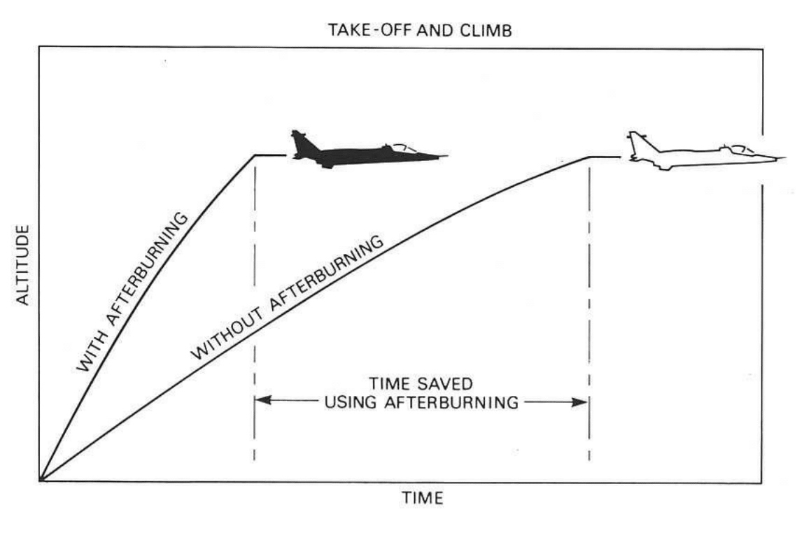
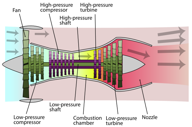
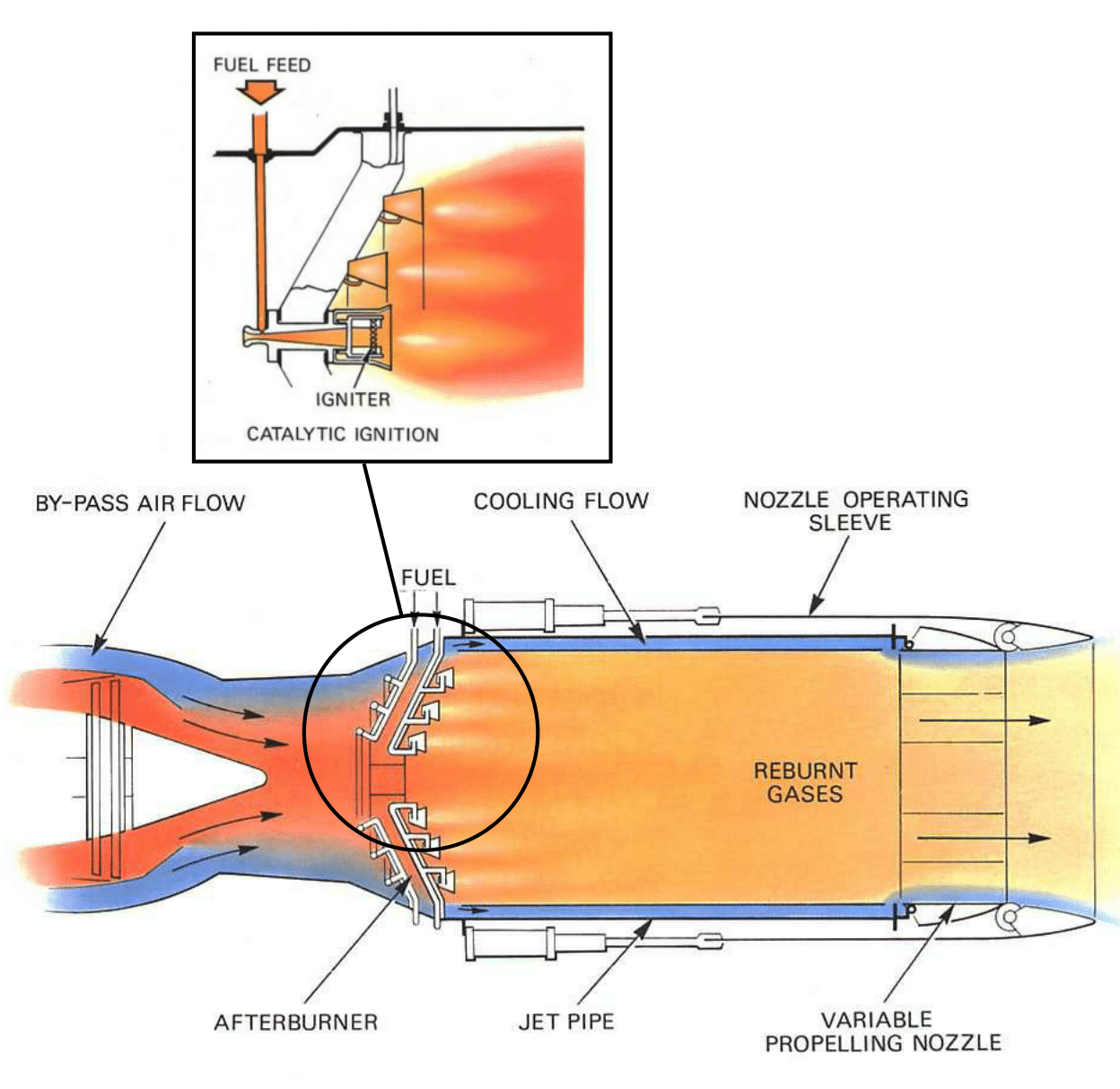
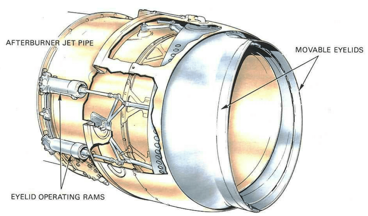
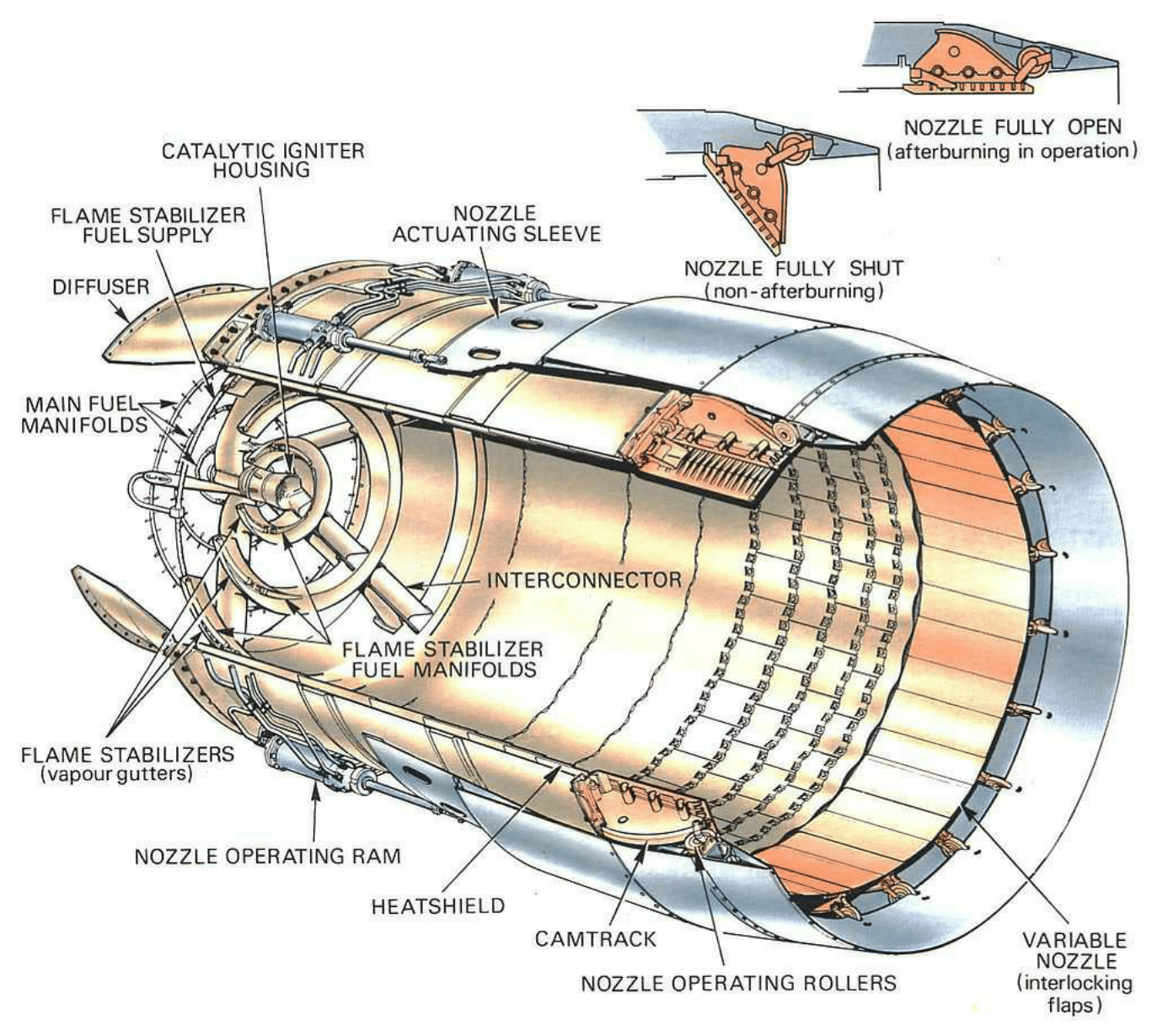
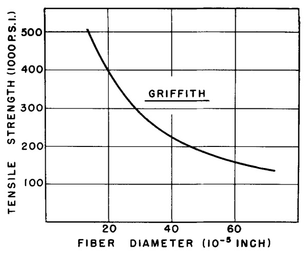
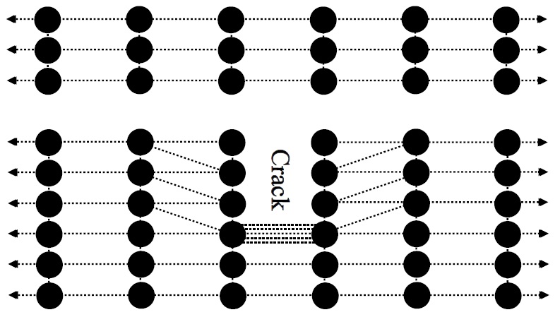


.jpg)


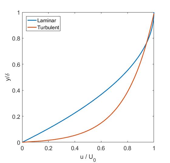
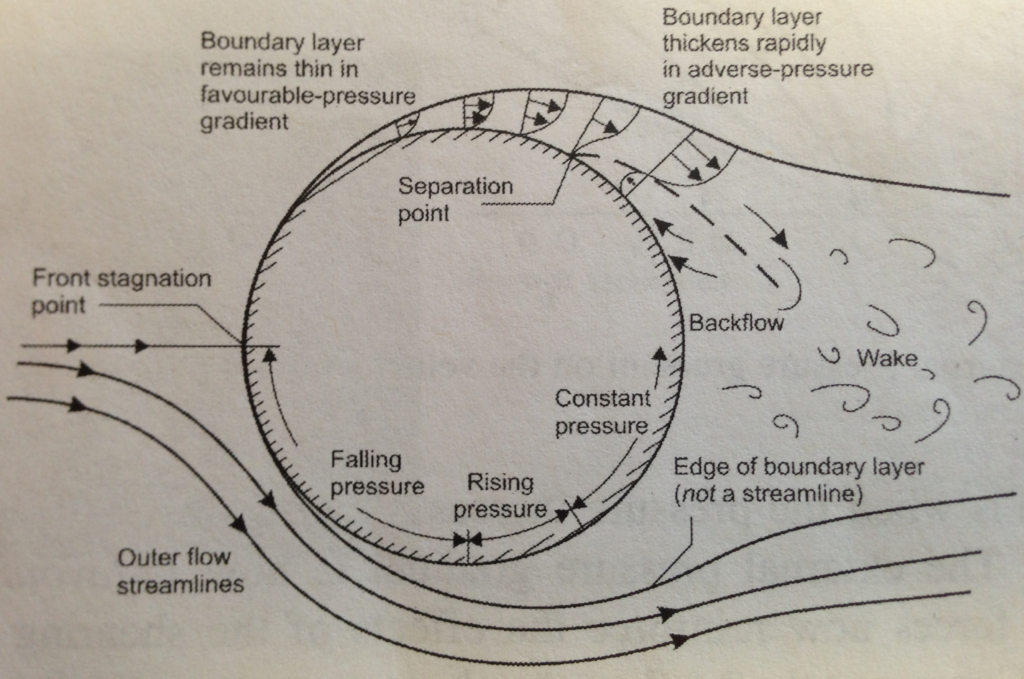
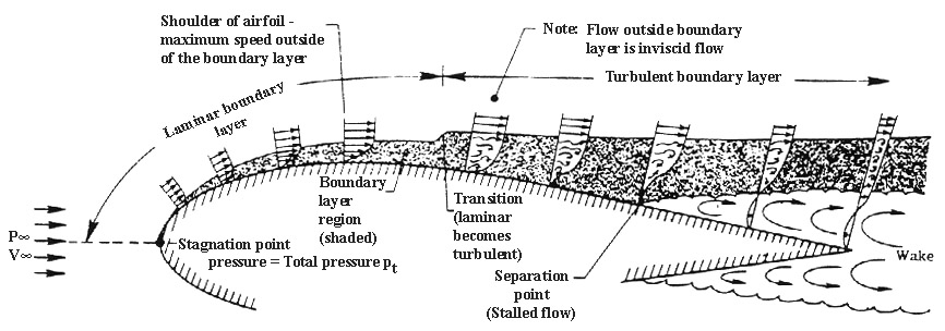


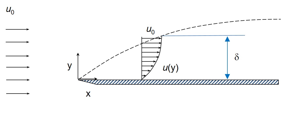
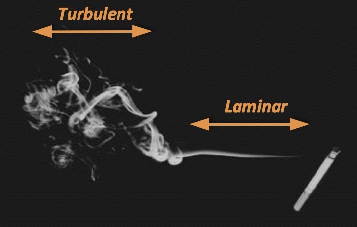

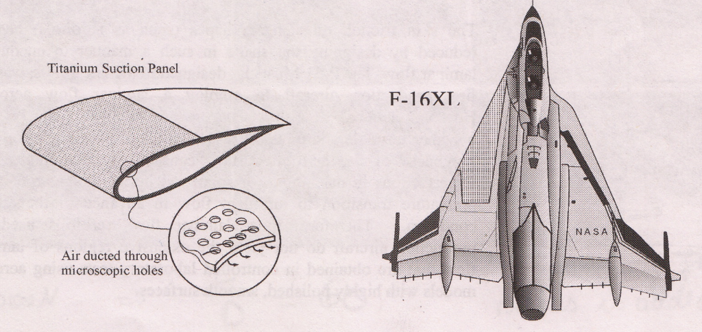
.jpg)