Tag: Aircraft

What Creates Lift – How Do Wings Work?
How airplanes fly is one of the most fundamental questions in aerospace engineering. Given its importance to flight, it is surprising how many different and oftentimes wrong explanations are being perpetuated online and in textbooks. Just throughout my time in school and university, I have been confronted with several different explanations of how wings create lift.

Most importantly, the equal transit time theory, explained further below, is taught in many school textbooks and therefore instils faulty intuitions about lift very early on. This is not necessarily because more advanced theories are harder to understand or require a lot maths. In fact, the theory that requires the simplest assumptions and least abstraction is typically considered to be the most useful.

In science, the simplicity of a theory is a hallmark of its elegance. According to Einstein (or Louis Zukofsky or Roger Sessions or William of Ockham…I give up, who knows), “everything should be made as simple as possible, but not simpler.” Hence, the strength of a theory is related to:
- The simplicity of its assumptions, ideally as few as possible.
- The diversity of phenomena the theory can explain, including phenomena that other theories could not explain.
Keeping this definition in mind, let’s investigate some popular theories about how aircraft create lift.

The first explanation of lift that I came across as a middle school student was the theory of “Equal Transit Times”. This theory assumes that the individual packets of air flowing across the top and bottom surfaces must reach the trailing edge of the airfoil at the same time. For this to occur, the airflow over the longer top surface must be travelling faster than the air flowing over the bottom surface. Bernoulli’s principle, i.e. along a streamline an increasing pressure gradient causes the flow speed to decrease and vice versa, is then invoked to deduce that the speed differential creates a pressure differential between the top and bottom surfaces, which invariably pushes the wing up. This explanation has a number of fallacies:
- There is no physical law that requires equal transit times, i.e. the underlying assumptions are certainly not as simple as possible.
- It fails to explain why aircraft can fly upside down, i.e. does not explain all phenomena.
As this video shows, the air over the top surface does indeed flow faster than on the bottom surface, but the flows certainly do not reach the trailing edge at the same time. Hence, this theory of equal transit times is often referred to as the “Equal Transit Time Fallacy”.

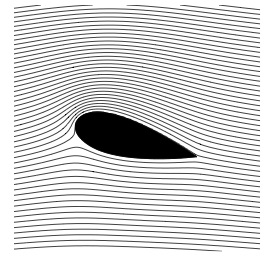
In order to generalise the above theory, while maintaining the mathematical relationship between speed and pressure given by Bernoulli’s principle, we can relax the initial assumption of equal transit time. If we start from a phenomenological observation of streamlines around an airfoil, as depicted schematically below, we see can see that the streamlines are bunched together towards the top surface of the leading edge, and spread apart towards the bottom surface of the leading edge. The flow between two adjacent streamlines is often called a streamtube, and the upper and lower streamtubes are highlighted in shades of blue in the figure below. The definition of a streamline is the line a fluid particle would traverse as it flows through space, and thus, by definition, fluid can never cross a streamline. As two adjacent streamlines form the boundaries of the streamtubes, the mass flow rate through each streamtube must be conserved, i.e. no fluid enters from the outside, and no fluid particles are created or destroyed. To conserve the mass flow rate in the upper streamline as it becomes narrower, the fluid must flow faster. Similarly, to conserve the mass flow rate in the lower streamtube as it widens, the fluid must slow down. Hence, in accordance with the speed-pressure relationship of Bernoulli’s principle, this constriction of the streamtubes means that we have a net pressure differential that generates a lift force.

Flow lines around a NACA 0012 airfoil at 11° angle of attack, with upper and lower streamtubes identified.

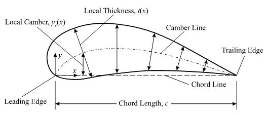
Of course, this theory does not explain why the upper streamtube contracts and the lower streamtube expands in the first place. An intuitive explanation for this involves the argument that the angle of attack obstructs the flow more towards the bottom of the airfoil than towards the top. However, this does not explain how asymmetric airfoils with pronounced positive camber at zero angle of attack, as shown in the figure below, create lift. In fact, such profiles were successfully used on early aircraft due to their resemblance to bird wings. Again, this theory does not explain all the physical phenomena we would like it to explain, and is therefore not the rigorous theory we are looking for.

Asymmetric airfoil with pronounced camber [1]

Another explanation that is often cited for explaining lift is that the airfoil pushes air downwards, i.e. there is a net change of momentum in the vertical plane between the leading and trailing edges of the airfoil, and by necessity of Newton’s third law, this creates a lift force. Any object that experiences lift must certainly conform to the reality of Newton’s third law, but referring only to the difference in start and end conditions ignores the potential complexity of flow that occurs between these two stations. Furthermore, the question remains through what net angle the flow is deflected? One straightforward answer is the angle of incidence of the airfoil, but this ignores the upwash ahead of the wing or anything that happens behind the wing. Hence, the simple explanation of “pushing air downwards”, however elegant and correct, is an integral approach that summates the fluid mechanics between leading and trailing edges and leaves little to say of what happens in between. Indeed, as will be shown below, upwash and flow circulation play an equally important role in creating lift.

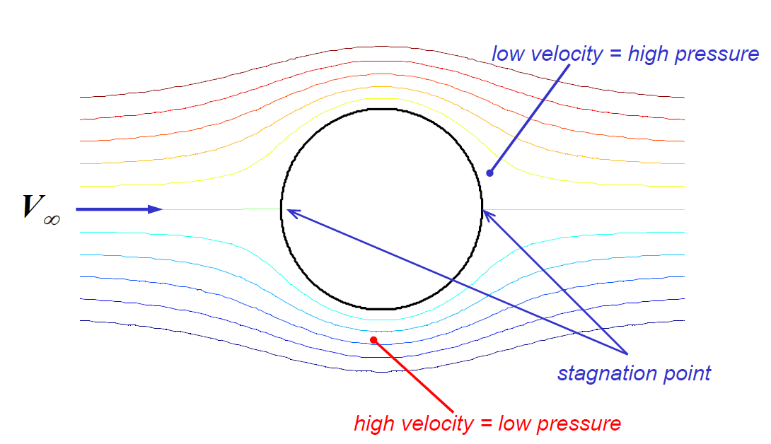
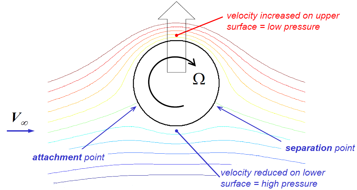
Indeed, we can imagine a flow around a 2D cylinder shown in the figure below. The flow is symmetric from left-to-right and top-to-bottom and experiences no lift. If we now start the cylinder spinning at the rate $\Omega$ in the clockwise direction shown, the velocity of air increases on the upper surface (reduced pressure) and reduces on the lower surface (higher pressure). This asymmetric flow top-to-bottom therefore creates lift. Note that the rotation of the cylinder has moved the stagnation point towards the rear end of the cylinder (where the bottom and top flows converge) downwards and therefore broken the symmetry of the flow. Hence, in this example, lift is created by a combination of a free-stream velocity and flow circulation, i.e. air is “spun up” and not necessarily just deflected downwards (in this example upwash ahead of the cylinder matches the downwash aft).

Flow around a cylinder

Flow around a rotating cylinder that induces lift

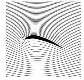
In the example above, lift was induced by creating an asymmetry in the curvature of the streamlines. In the stationary cylinder we had streamlines curving in one direction on the top surface, and by the same amount in the opposite direction on the bottom surface. Rotating the cylinder created an asymmetry in streamline curvature between the top and bottom surfaces (more curvature upwards then curvature downwards). We can create a similar asymmetry in the flow with a stationary cylinder by placing a small sharp-edged flap at the rear edge and positioned slightly downwards. Real viscous flow might not necessarily flow as smoothly around the little flap as shown in the diagram below, but this mental model is a neat tool to imagine how we can morphologically transition from a rotating cylinder that produces lift to an airfoil. This is shown via the series of diagrams below. This series of pictures shows that an airfoil creates a smoother variation in velocity than the cylinder, which leads to a smaller chance of boundary layer separation (a source of drag and in the worst-case scenario aerodynamic stall). A similar streamline profile could also be created with a symmetric airfoil that introduces asymmetry into the flow by being positioned at a positive angle of attack.

The reason why differences in streamline curvature induce lift is addressed in a journal paper by Prof Holger Babinsky, which is free to download. If we consider purely stead-state flow and neglect the effects of gravity, surface tension and friction we can derive some very basic, yet insightful, equations that explain the induced pressure difference. Quite intuitively this argument shows that a force acting parallel to a streamline causes the flow to accelerate or decelerate along its tangential path, whereas a force acting perpendicular to the flow direction causes the streamline to curve.

The first case is described mathematically by Bernoulli’s principle and depicted in the figure below. If we imagine a small fluid particle of finite length l situated in a field of varying pressure, then the front and back surfaces of the particle will experience different pressures. Say the pressure increases along the streamline, then the force acting on the front face pointing in the direction of motion is greater than the force acting on the rear surface. Hence, according to Newton’s second law, this increasing pressure field along the streamline causes the flow speed to decrease and vice versa. However, this approach is valid only along a single streamline. Bernoulli’s principle can not be used to relate the speed and pressures of adjacent streamlines. Thus, we can not use Bernoulli’s principle to compare the flows on the bottom and top surfaces of an airfoil, and therefore can say little about their relative pressures and speeds.

Flow along a straight streamline [2]

However, consider the curved streamlines shown in the figure below. If we assume that the speed of the particle travelling along the curved streamline is constant, then Bernoulli’s principle states that the pressure along the streamline can not change either. However, the velocity vector v is changing, as the direction of travel is changing along the streamline. According to Newton’s second law, this change in velocity, i.e. acceleration, must be caused by a net centripetal force acting perpendicular to the direction of the flow. This net centripetal force must be caused by a pressure differential on either side of the particle as we have ignored the influence of gravity and friction. Hence, a curved streamline implies a pressure differential across it, with the pressure decreasing towards the centre of curvature.

Flow along a curved streamline [2]

Mathematically, the pressure difference across a streamline in the direction n pointing outwards from the centre of curvature is

$\frac{\mathrm{d}p}{\mathrm{d}n} = \rho \frac{v^2}{R}$

where R is the radius of curvature of the flow and $\rho$ is the density of the fluid.

One positive characteristic of this theory is that it explains other phenomena outside our interest in airfoils. Vortices, such as tornados, consist of concentric circles of streamlines, which suggests that the pressure decreases as we move from the outside to the core of the vortex. This observation agrees with our intuitive understanding of tornados sucking objects into the sky.

With this understanding we can now return to the study of airfoils. Consider the simple flow path along a curved plate shown in the figure below. At point A the flow field is unperturbed by the presence of the airflow and the local pressure is equal to the atmospheric pressure $p_{atm}$ . As we move down along the dashed curve we see that the flow starts to curve around the curved plate. Hence, the pressure is decreasing as we move closer to the airfoil surface and $p_B < p_{atm}$ . On the bottom half the situation is reversed. Point C is again undisturbed by the airflow but the flow is increasingly curved as me closer to D. However, when moving from C to D, the pressure is increasing because pressure increases moving away from the centre of curvature, which on the bottom of the airfoil is towards point C. Thus, $p_D > p_{atm}$ and by the transitive property $p_B < p_D$ such that the airfoil experiences a net upward lift force.

Flow around a curved airfoil [2]

From this exposition we learn that any shape that creates asymmetric curvature in the flow field can generate lift. Even though friction has been neglected in this analysis, it is crucial in forcing the fluid to adhere to the surfaces of the airfoil via a viscous boundary layer. Therefore, the inclusion of friction does not change the theory of lift due to streamline curvature, but provides an explanation for why the streamlines are curved in the first place.

A couple of interesting observations follow from the above discussion. Nature typically uses thin wings with high camber, whereas man-made flying machines typically have thicker airfoils due to their improved structural performance, i.e. stiffness. In the figure below, the deep camber thinner wing shows highly curved flow in the same direction on both the top and bottom surfaces.

Deep camber thin wing with high lift [2]

Shallow camber thick wing with less lift [2]

The more shallow camber thicker wing has flow curved in two different directions on the bottom surface and will therefore result in less pressure difference between the top and bottom surfaces. Thus, for maximum lift, the thin, deeply cambered airfoils used by birds are the optimum configuration.

In conclusion, we have investigated a number of different theories explaining how lift is created around airfoils. Each theory was investigated in terms of the simplicity and validity of its underlying assumptions, and the diversity of phenomena it can describe. The theories based on Bernoulli’s principle, such as the equal transit time theory and the contraction of streamtubes theory, were either based on faulty initial assumptions, i.e. equal time, or failed to explain why streamtubes should contract or expand in the first place. The theory based on airfoils deflecting airflow downwards is theoretically accurate and correct (Newton’s third law: changes in fluid momentum over a control volume including the airfoil lead to a reactive lift force), but by being an integral approach it is not helpful in explaining what occurs between the leading and trailing edges of the airfoil (e.g. upwash is also a contributing factor to lift).

A more intricate theory is that curved bodies induce curved streamlines, as the inherent viscosity of the fluid forces the fluid to adhere to the surface of the body via a boundary layer. The centripetal forces that arise in the curved flow lead to a drop in pressure across the streamlines towards the centre of curvature. This means that if a body leads to asymmetric curved streamlines across it, then the induced pressure differential arising from the asymmetry induces a net lift force.

Edits and Acknowledgments

A previous version of this article referenced a misleading and incorrect example of a highly cambered airfoil as a counterexample to the theory of airfoils deflecting airflow downwards and the theoretical explanation using control volumes. Dr Thomas Albrecht of Monash University pointed this error out to me (see the discussion in the comments) and his contribution in improving the article is gratefully acknowledged.

Photo credit

[1] DThanhvp. Photobucket. http://s37.photobucket.com/user/DThanhvp/media/American.jpg.html

[2] Babinsky, H. (2003). How do wings work?. Physics Education 38(6) pp. 497-503. URL: http://iopscience.iop.org/article/10.1088/0031-9120/38/6/001/pdf;jsessionid=64686DBCB81FEB401CFFB87E18DFE6DA.c1
October 10, 2015
Big Data in Aerospace

“Big data” is all abuzz in the media these days. As more and more people are connected to the internet and sensors become ubiquitous parts of daily hardware an unprecedented amount of information is being produced. Some analysts project 40% growth in data over the next decade, which means that in a decade 30 times the amount of data will be produced than today. Given this this trend, what are the implications for the aerospace industry?

Big data: According to Google a “buzzword to describe a massive volume of both structured and unstructured data that is so large that it’s difficult to process using traditional database and software techniques.”

Fundamentally, big data is nothing new for the aerospace industry. Sensors have been collecting data on aircraft for years ranging from binary data such as speed, altitude and stability of the aircraft during flight, to damage and crack growth progression at service intervals. The authorities and parties involved have done an incredible job at using routine data and data gathered from failures to raise safety standards.

What exactly does “big data” mean? Big data is characterised by a data stream that is high in volume, high velocity and coming from multiple sources and in a variety of forms. This combination of factors makes analysing and interpreting data via a live stream incredibly difficult, but such a capability is exactly what is needed in the aerospace environment. For example, structural health monitoring has received a lot of attention within research institutes because an internal sensory system that provides information about the real stresses and strains within a structure could improve prognostics about the “health” of a part and indicate when service intervals and replacements are needed. Such a system could look at the usage data of an aircraft and predict when a component needs replacing. For example, the likelihood that a part will fail could be translating into an associated repair that is the best compromise in terms of safety and cost. Furthermore, the information can be fed back to the structural engineers to improve the design for future aircraft. Ideally you want to replicate the way the nervous system uses pain to signal damage within the body and then trigger a remedy. Even though structural health monitoring systems are feasible today, analysing the data stream in real time and providing diagnostics and prognostics remains a challenge.

Other areas within aerospace that will greatly benefit from insights gleaned from data streams are cyber security, understanding automation and the human-machine interaction, aircraft under different weather and traffic situations and supply chain management. Big data could also serve as the underlying structure that establishies autonomous aircraft on a wide scale. Finally, big data opens the door for a new type of adaptive design in which data from sensors are used to describe the characteristics of a specific outcome, and a design is then iterated until the desired and actual data match. This is very much an evolutionary, trail-and-error approach that will be invaluable for highly complex systems where cause and effect are not easily correlated and deterministic approaches are not possible. For example, a research team may define some general, not well defined hypothesis about a future design or system they are trying to understand, and then use data analytics to explore the available solutions and come up with initial insights into the governing factors of a system. In this case it is imperative to fail quickly and find out out what works and what does not. The algorithm can then be refined iteratively by using the expertise of an engineer to point the computer in the right direction.

Thus, the main goal is to turn data into useful, actionable knowledge. For example in the 1990’s very limited data existed in terms of understanding the airport taxi-way structure. Today we have the opposite situation in that we have more data than we can actually use. Furthermore, not only the quantity but also quality of data is increasing rapidly such that computer scientists are able to design more detailed models to describe the underlying physics of complex systems. When converting data to actionable information one challenge is how to account for as much of the data as possible before reaching a conclusion. Thus, a high velocity, high volume and diverse data stream may not be the most important characteristic for data analytics. Rather it is more important that the data be relevant, complete and measurable. Therefore good insights can also be gleaned from smaller data if the data analytics is powerful.

While aerospace is neither search nor social media, big data is incredibly important because the underlying stream from distributed data systems on aircraft or weather data systems can be aggregated and analysed in consonance to create new insights for safety. Thus, in the aerospace industry the major value drivers will be data analytics and data science, which will allow engineers and scientists to combine datasets in new ways and gain insights from complex systems that are hard to analyse deterministically. The major challenge is how to upscale the current systems into a new era where the information system is the foundation of the entire aerospace environment. In this manner data science will transform into a fundamental pillar of aerospace engineering, alongside the classical foundations such as propulsion, structures, control and aerodynamics.

March 26, 2015
The Evolution of Airplanes
Adrian Bejan is a Professor of Mechanical Engineering and Materials Science at Duke University and as an offshoot from his thermodynamics research he has pondered the question why evolution exists in natural i.e. biological and geophysical, and man-made, i.e. technological, realms. To account for the progress of design in evolution Prof. Bejan conceived the constructal law, which states that

For a finite-size flow system to persist in time (to live), its configuration must evolve (freely) in such a way that it provides easier access to the currents that flow through it.

In essence a new technology, design or species emerges so that it offers greater access to the resources that flow i.e. greater access to space and time. The unifying driver behind the law is that all systems that output useful work have a tendency to produce and use power in the most efficient manner.

The Lena Delta. Photo Credit Wikipedia [1]

Given Prof. Bejan’s specialty in thermodynamics it is no surprise that the law uses the analogy of a flow system to describe the evolution of design. In nature the branches of rivers carry water, nutrients and sediments to the sea, and if given enough freedom, over time evolve into a river delta that provides a source of life for an entire area. Similarly, our lungs facilitate flow of chemical energy between air and blood and have evolved into a complex multi-branch system that aims to improve the flow of currents within it.

A difficulty in studying natural evolution is that it occurs on a time-scale much greater than our lifetime. However, in a recent study published in the Journal of Applied Physics Prof. Bejan and co-workers show that the shorter technological evolution of airplanes allows us to witness the phenomenon from a bird’s-eye view. Interestingly, as a “flying machine species” the evolution of airplanes follows the same physical principles of evolution that are observed in birds and that can be captured elegantly using the constructal law. For example, the researchers found that
- Larger airplanes travel faster. In particular the flight velocity of aircraft is proportional to its mass raised to the power 1/6, i.e. $V = k M^{1/6}$
- The engine mass is proportional to body mass, much in the same way that muscle mass and body mass are related in animals
- The range of an aircraft is proportional to its body mass, just as larger rivers and atmospheric currents carry mass further, and bigger animals travel farther and live longer.
- Wing-span is proportional to fuselage length (body length), and both wing and fuselage profiles fit in slender rectangles of aspect ratio 10:1
- Fuel load is proportional to body mass and engine mass, and these scale in the same way as food intake and body mass in animals.
This overall trend is depicted nicely in Figure 1 which shows the size of new airplane models against the year they were put into service. It is evident that the biggest planes of one generation are surpassed by even bigger planes in the next. Based on economical arguments it can be assumed that each model introduced was in some way more efficient in terms of passenger capacity, speed, range, i.e. cost-effectiveness than the previous generation of the same size. Thus, in terms of the constructal law the spreading of flow is optimised and this appears to be closely matched with the airplane size and mass. Similarly, Figure 2 shows that both birds and aircraft evolve in the same way in that the bigger fly faster. Thus, the evolution of natural and technological designs seems to have converged on the same scaling rules. This convergent design is also evident in the number of new designs that appear over time. At the start of flight the skies were dominated by swarms of insects of very different design. These were followed by a smaller number of more specialised bird species and today by even fewer “aircraft species”. Combining these two ideas of size and number, it seems that the new are few and large, whereas the old are many and small.

Figure 1. Evolution of airplane mass versus time [2]

Figure 2. Evolution of animal flight speed versus body mass [2]

The key question is why engines, fuel consumption or wing sizes should have a characteristic size?

Any vehicle that moves and consumes fuel to propel it depends on the function of specific organs, say the engines or fuel ducts, that interact with the the fuel. Because there is a finite size constraint for all these organs the vehicle performance is naturally constrained in two ways:
1. Resistance, i.e. friction and increasing entropy within the organs. This penalty reduces for larger organs as larger diameter fuel ducts have less flow resistance and larger engines encounter less local flow problems. Thus, larger is generally better
2. On the flip side the larger the organ the more fuel is required to move the whole vehicle. But the more fuel is added the more the overall mass is increased and the more fuel you need, and so on. This suggests that smaller is better.
From this simple conflict we can see that a size compromise needs to be reached, not too small and not too large, but just right for the particular vehicle. In essence what this boils down to is that larger organs are required on proportionally large vehicles and small organs on small vehicles. Thus, as more and more people intend to travel and move mass across the planet the old design based on small organs becomes imperfect and a more efficient, larger design for the new circumstances is required.

Overall, the researchers conclude that the physical principles of evolution define the viable shape of an aircraft. Thus, the fuselage and the wing must be slender, the fuselage cross-section needs to be round and the wing span must be proportional to the fuselage length. A famous outlier that broke with these evolutionary trends of previous successful airplanes was the Concorde with its long fuselage, massive engines and short wingspan. Rather than attempting to achieve an overall superior solution the designers attempted to maximise speed, and thereby compromised passenger capacity and fuel efficiency. Only 20 units were ever produced and due to lack of demand and safety concerns the Concorde was retired in 2003. Current aircraft evolution manifested in the Boeing 787 Dreamliner, 777X and Airbus A350 XWB are rather based on combining successful architectures of the past and with new concepts, that allow the overall design to remain within the optimal evolutionary constraints. Thus, it is no surprise that in an attempt to make aircraft larger and at the same time more efficient, the current shift from metal to carbon fibre construction is what is needed to elevate designs to a higher level.

References

[1] http://en.wikipedia.org/wiki/Lena_Delta_Wildlife_Reserve#mediaviewer/File:Lena_River_Delta_-_Landsat_2000.jpg

[2] Bejan, A., Charles, J.D., Lorente, S. The evolution of airplanes. Journal of Applied Physics, 116. 2014.
December 9, 2014
Loads Acting on Aircraft

The flight envelope of an aeroplane can be divided into two regimes. The first is rectilinear flight in a straight line, i.e. the aircraft does not accelerate normal to the direction of flight. The second is curvilinear flight, which, as the name suggests, involves flight in a curved path with acceleration normal to tangential flight path. Curvilinear flight is often known as manoeuvring and is of greater importance for structural design since the aerodynamic and inertial loads are much higher than in rectilinear flight.

As the aircraft moves relative to the surrounding fluid a pressure field is set up over the entire aircraft, and not only over the wings, that acts to keep the aircraft afloat. This aerodynamic pressure always acts normal to the outer contour of the skin but the resultant force can be resolved into two forces acting tangential and normal to the direction of flight. The sum of the forces normal to the direction of flight give rise to the lift force L, which offsets the weight of the aircraft i.e. offsets the weight of the aircraft W. The tangential components give the resultant drag force D, which in powered flight must be overcome by the propulsive force F. The resultant force F includes the thrust generated by the engines, the induced drag of the propulsive system and the inclination of the line of thrust to the direction of flight. In basic mechanics the aircraft is simplified into a point coincident with the centre of gravity (CG) of the aircraft with all forces assumed to act through the centre of gravity. If the net resultant of a force is offset from the CG then a resultant moment will also act on the aircraft. For example, the lift generated by the wings is generally offset from the centre of gravity of the aircraft and may thus produce a net pitching moment that has to be offset by the control surfaces. Figure 1 below shows as a simplified free body diagram of an aircraft in level flight, climb and descent.

Fig. 1. Free body diagram of aircraft in flight (1)

Note that the lift is only equal and opposite to the weight in steady and level flight, thus:

$F=D$ and $L=W$

In steady descent and steady climb the lift component is less than the weight, since only a component of the weight acts normal to the direction of flight and because by definition lift is always normal to both drag and thrust. Also in climbing the thrust must be greater than the drag to overcome the component of weight acting against the direction of flight and vice versa in descent. Thus in a climb:

$L = W \cos \gamma_c$ and $F = D + W \sin \gamma_c$

and in descent

$L = W \cos \gamma_d$ , $F = D – W \sin \gamma_d$

This situation is schematically represented in Figure 1 by the relative sizes of the different arrows. In general we can imagine the weight being balanced by the lift force L and the difference between the thrust F and the drag D. A bit of manipulation of the two equations for climb or descent above gives the same expression,

$L^2 + (F-D)^2 = W^2 \cos^2 \gamma_c + W^2 \sin^2 \gamma_c$

such that,

$W = \sqrt{L^2 + (F-D)^2}$

The latter expression is clearly obtained if Pythagoras’ rule is applied to the vector triangles that include (F-D) and L in Figure 1.

Figure 1 also shows velocity diagrams depicting the relationship between true air speed V, tangential to the direction of flight, and the rates of climb and descent $v_c$ and $v_c$ , respectively. We can combine these velocity triangles with the forces triangles to obtain simple equations for the rates of climb and descent,

$\sin \gamma_c = \frac{F-D}{W}$ and $\sin \gamma_c = \frac{v_c \ or \ v_d}{V}$

such that $v_c$ or $v_d = \frac{F-D}{W} V$ .

This expression can also be used to gain some insight into the driving factors behind gliding flight. In this case the net propulsive force F is zero such that the expression becomes, $v_d = -\frac{D}{W} V$ which may be approximated to $v_d = -\frac{D}{L} V$ since the angle of descent in gliding is typically very shallow. Therefore the gliding efficiency of a sailplane depends on maximising the lift to drag ratio L/D. If the ascending thermals are equal to or greater than this rate of descent than the glider can continuously maintain or even gain in altitude.

An aircraft may of course increase its speed along the direction of rectilinear flight in which case the thrust force F must be greater than the vector sum of the drag and the component of the weight. A more interesting scenario are accelerated flight where the acceleration occurs as a result in change in direction rather than a change in speed. By definition, in vector mechanics a change in direction is a change in velocity and therefore defined as acceleration, even if the magnitude of the speed does not change. A change in the flight path is achieved by changing the magnitude of the overall lift component or by differences in lift between the two wings, away from the equilibrium condition depicted in Figure 1. This change can either be obtained by a change in true airspeed or by changing the angle of attack of the wings relative to the airflow. Consider the simple banked turn in Figure 2 below.

Fig. 2. Free Body Diagram of an aircraft in a banked turn (1)

As the aircraft banks the lift force normal to the wings is turned through an angle $\theta$ from the vertical weight vector. Since the centripetal acceleration acts horizontally and the weight acts vertically we can use simple trigonometric relations to find the radius of turn: $\tan \theta = \frac{F_{centripetal}}{W} = \frac{m V^2 / R }{m g}$ such that $R = \frac{V^2}{g \tan \theta}$ . It is also obvious that the more steeply banked the turn the more lift will be required from the wings since,

$L = \frac{W}{\cos \theta}$

such that increase in engine power is needed to maintain constant speed under this flight condition. This is one of the reasons why fighter jets that require manoeuvres with very tight radii have such short and stubby wings. Small radii if turn R and thus high banking angles $\theta$ require increases in lift and therefore increase the bending moments acting on the wings.

In reality the airplane is subjected to a large variety of different combinations of accelerations (rolls, pull-ups, push-overs, spinning, stalling , gusts etc.) at different velocities and altitudes. In classical mechanics free fall is expressed as having an acceleration of -1g and level flight is denoted as 0g. The aeronautical engineer differs from this convention in order to make the comparison between lift and weight simpler. This means that free fall is denoted by 0g and level flight by 1g. The ratio between lift and aircraft weight is called the load factor n, where $n = \frac{L}{W}$ , i.e. n = 0 for free fall, n = 1 for level flight, n > 1 to pull out of a dive and n < 1 to pull out of a climb. The overall load spectrum of an aircraft is captured graphically by so called velocity – load factor (V-n) curves. The outline of these diagrams are given by the possible combinations of load factor and velocity than an aircraft will be expected to cope with. For example Figure 3a shows the basic V-n diagram for symmetric flight (asymmetric envelopes exist for rolls etc. but are not covered here).

Fig. 2 The a) basic manoeuvre and b) gust flight envelopes (1)

The envelope is constructed from the positive and negative stall lines which indicate, respectively, the maximum and minimum load that can be achieved because of the inability of the aircraft to produce any more lift. Thus,

$L = n W = \frac{1}{2}C_{L_{max}} \rho V^2 S$

where $\rho$ is the density of the surrounding air and $S$ is the wing surface area. The limiting factor $n_l$ also known as the maximum expected service load is defined by $n_l = 2.1 + \frac{24 000}{W + 10 000}$ or 2.5, whichever is greater, with W the max take-off weight.

$V_A$ , $V_C$ and $V_D$ are defined as the maximum manoeuvre speed ( the speed above which it is unwise to make full application of any single flight control), the design cruise speed and the maximum dive speed, respectively. The intersection between the horizontal line $n=1$ and the left curve of the envelope is also of special significance since it represents the stall speed at level flight. In general the limit load factor must be tolerable without detrimental permanent deformation. The aircraft must also support an ultimate load (=limit load x safety factor) for at least 3 seconds. The safety factor is generally taken to be 1.5.

Finally, Figure 3b shows a typical gust envelope. A gust alters the angle of attack of the lifting surfaces by an amount equal to $\tan^{-1} (w/V)$ where w is the vertical gust velocity. Since the lift scales with the angle of attack up to the point of aerodynamic stall, the inertia forces applied to structure are altered by the gust winds. The gust envelope is constructed with the same stall lines as the basic manoeuvre envelope and different gust lines are drawn radiating from n = 1 at V = 0. Note that the design gust intensities reduce as the velocity increases, with the intention that the aircraft is flown accordingly. In the gust envelope $V_A$ is replaced with $V_B$ , representing the design speed at maximum gust intensity.

References

(1) Stinton, D. The Anatomy of the Airplane. 2nd Edition. Blackwell Science Ltd. (1998).

February 2, 2014
Breguet Range Equation

There is a saying that your audience will halve for every equation you put in a piece of writing. Well, in this case I am going to make an exception and go through the detailed derivation of the Breguet Range equation. The reason for doing this is that the maths is not very difficult but the implications of the equation are known to every pilot on earth and everyone interested in flight should know about it. Simply put, the Breguet range equation tells engineers how far and airplane can fly given a certain set of parameters, and therefore greatly influences the design of modern jet engines and airframes.

A central aspect of flying further for the same amount of fuel is maximising the lift to drag ratio of your wings and airframe. Optimising this ratio gives the maximum aircraft weight (=lift at steady horizontal flight) that can be kept in the air for a given amount of engine thrust (=drag at steady horizontal flight). However, this parameter is not the primary optimum for commercial flight. Instead one wants to fly the furthest possible distance with one fuel filling. Thus to achieve the maximum possible range the quantity to be optimised is the product of flight speed (U) with lift (L) to drag (D) ratio [latex]\frac{UL}{D}[/latex]. For most long-haul journeys (~12 hours) the most time consuming part of the journey, and therefore most critical for fuel consumption is the cruise condition. During cruise conditions the band of altitudes that the airliner travels through does not vary greatly such that the local speed of sound [latex]U_s=\sqrt{\gamma R T}[/latex] where T is the local static temperature, does not vary greatly. Consequently optimising the Mach Number [latex]M=\frac{U}{\sqrt{\gamma R T}}[/latex] times the lift to drag ratio [latex]\frac{ML}{D}[/latex] is virtually the same.

Figure 1 shows experimental data of this parameter versus the lift-coefficient [latex]C_L = \frac{2L}{\rho v^2 S}[/latex] for a Boeing 747-400 at 35,000 ft. At each Mach number L/D rises to a maximum until further increase in lift coefficient leads to stall of the aerofoil. At lower flight speeds the boundary layer separation will occur naturally towards the trailing edge but as we approach a flight speed of Mach 1 shock waves also come into play. The graph shows that for all cruise speeds the optimum value of [latex]\frac{ML}{D}[/latex] occurs at a lift coefficient of about 0.5. The wing area S of an aeroplane is set largely by conditions at take-off and landing, such that it is hard to continually operate at a lift coefficient of 0.5 as the weight and therefore lift of the aeroplane decreases as fuel is burnt. To operate as close to optimum on can therefore decrease v, not very attractive, or decrease the density [latex]\rho[/latex] by flying at higher altitudes. Large airliners therefore typically start cruise at 31 000 ft or higher and then increase altitude in steps to fly at the optimum [latex]\frac{ML}{D}[/latex].

Fig. 1. Mach number x lift-drag versus lift coefficient for various flight Mach numbers (1).

The global maximum is achieved for a cruise speed of M = 0.86. Beyond this point [latex]\frac{ML}{D}[/latex] can be seen to fall precipitously. Since the air accelerates over the top surface of the aerofoil flight speeds close to Mach 1 can lead to local pockets of supersonic flow over the airflow. At some point these supersonic pockets terminate in a lambda shock wave across which the local air pressure increases to obey the law of thermodynamics. This increase in pressure exacerbates the adverse pressure gradient along the length of the aerofoil, leading to earlier boundary layer separation and an induced increase in drag. Furthermore, the separation caused by shock waves leads to buffeting and control problems. For this reason the typical Mach Number during cruise is set around 0.85.

The next time you fly you could easily check this using one of the onboard screens that display flight data. Take the formula [latex]M=\frac{U}{\sqrt{\gamma R T}}[/latex], and set U equal to flight speed in meters/second (= km/hr divided by 3.6), ratio of specific heat capacity [latex]\gamma = \frac{c_p}{c_v}=1.4[/latex], gas constant [latex]R= 287.05 J/(kg K)[/latex] and local temperature T in Kelvin = T in °C +273. Alternatively replacing all values in the equation we get [latex]M=\frac{U (km/hr)}{72.17*\sqrt{T(C) + 273}}[/latex]. Typical flight conditions are 880 km/hr at -60°C giving a Mach Number of 0.83.

The conventional measure of the amount of fuel used compared to the thrust produced is the specific fuel conusmption (SFC). The SFC is the fuel mass-flow rate divided by the thrust produced and therefore has units of kg/(Ns). At cruise, the rate of change of weight (dW/dt) is proportional to the fuel mass-flow rate , [latex]\dot{m}_f[/latex], such that,

[latex]\frac{\mathrm{d}W}{\mathrm{d}t} = -\dot{m}_fg[/latex]

The negative sign indicates that the weight of the aeroplane is decreasing with time as fuel is burnt. The SFC is,

[latex]SFC = \frac{\dot{m}_f}{F}[/latex]

and since F = D for horizontal cruise we have,

[latex]\frac{\mathrm{d}W}{\mathrm{d}t} = -Dg(SFC)[/latex]

Since W=L for horizontal cruise,

[latex]\frac{\mathrm{d}W}{\mathrm{d}t} = -\frac{Wg(SFC)}{L/D}[/latex]

For constant speed U the distance travelled is dx = U*dt, hence

[latex]\frac{\mathrm{d}W}{W} = -\frac{g(SFC)}{UL/D}\mathrm{d}x[/latex]

If SFC, U and L/D are constant this expression can be integrated to give the final result,

[latex]\ln\left( \frac{W_2}{W_1} \right) = -\frac{g(SFC)}{UL/D} \Delta x \quad \text{or} \quad \Delta x = -\frac{UL/D}{g(SFC)} * \ln\left( \frac{W_2}{W_1} \right)[/latex]

where [latex]W_1 \text{ and } W_2[/latex] are the initial and final weights during cruise. This equation is known as the Breguet Range equation. We discussed before that [latex]\frac{UL}{D}[/latex] should be optimised to increase range. However, it can be noted that the range is inversely proportional to the SFC and since SFC is also a function of the flight speed U the situation is a bit more complicated. In reality the aim is to maximise the ratio of [latex]\frac{UL}{(SFC)D}[/latex]. Of course SFC also depends on the efficiency of the jet engines, which has been discussed in a series of previous posts (1,2,3). Furthermore, the structural weight is crucial forming a large part of [latex]W_2[/latex]. Finally the aerodynamic profile of the whole aircraft has to be optimised in order to reduce drag and thereby decrease the thrust F required to overcome it.

References

(1) Cumpsty, N.A. (2003). Jet Propulsion: A Simple Guide to the Aerodynamic and Thermodynamic Design and Performance of Jet Engines. Cambridge University Press.

June 9, 2013
Bio-mimetic Drag Reduction – Part 2: Aero- and Hydrodynamics
Part 1 of this blog series outlined the different sensing mechanisms that aquatic animals possess to create spatial images of the flow fields around them. In summary fish were found to possess a network of mechanosensors distributed over their bodies called the lateral line. The lateral line consists of two separate sensory subsystems:
- a system of velocity-sensitive superficial neuromasts that responds to slow, uniform motions and that integrates large scale stimuli at the periphery such as constant currents
and
- a system of acceleration- or pressure-gradient-sensitive canal neuromasts that responds to rapidly changing motions and gives the fish the opportunity to orient towards sources such as prey or optimize swimming speed or tail-flapping frequency.
In this post I will give a brief overview of general hydrodynamic theory and specifically the flow patterns that swimming fish are expected to sense with their network of neuromasts.

When a body moves relative to a fluid, a boundary layer exists close to the wall because of the “no slip” condition, which arises from the inherent stickiness or so-called viscosity of the fluid. Therefore, fluid in direct contact with the wall adheres to the surface while fluid further away is slowed due to the frictional forces arising from viscosity. This results in a thin layer of fluid where the velocity increases in a U-profile from zero at the wall to the free stream velocity some distance d from the surface; defined as the boundary layer thickness (Figure 1).

Fig. 1. Boundary layer close to a surface (1).

Generally speaking fluid flow can be classified as either laminar or turbulent. In laminar flow (derived from “lamina” meaning finite layers) the fluid moves in lamina or layers of finite speed and with no mixing of the fluid perpendicular to the wall i.e. across layers. As the name suggest in turbulent flow everything is a bit more chaotic with active mixing of the fluid and momentum transfer throughout the boundary layer (Figure 2).

Fig. 2. Laminar and Turbulent Boundary Layer (2).

The type of flow depends on the shape of the body, upstream history of the flow, surface roughness and most importantly the Reynolds Number. The Reynold’s number Re is a non-dimensional ration of the inertial forces to the viscous forces arising in the fluid defined by,

where p is the density of the fluid, v the velocity, u the viscosity and D a characteristic dimensions that describes the body under investigation. At certain critical Reynold’s number there is a natural transition from laminar to turbulent flow. For example if we consider the plate in Figure 3 we can observe that a boundary layer forms close to the surface once the flow encounters the leading edge of the plate. Initially the boundary layer thickness is very small but as we proceed along the length of the plate the boundary layer becomes thicker as increasingly more fluid is slowed down by the frictional effects of viscosity. The characteristic dimension for Re in this case is the distance l from the leading edge. This means that close to the leading edge where l is small the flow will be laminar while at a certain distance l_critical the critical value of Re is reached an the flow naturally transitions to turbulent flow.

Fig. 3. Laminar to turbulent transition over flat plate (2).

Now there are two major types of drag: skin friction drag, which is similar to the friction force you feel when you rub your hand over a table-top, and pressure drag, which results from a difference in fluid pressure between the front and rear of the body. As intuitively expected skin friction drag depends on the viscosity (stickiness) of the fluid but also the relative difference in velocity between different layers of fluid. Figure 3 shows that in a turbulent boundary layer the flow velocity increases more rapidly as we move away from the wall compared to a laminar boundary layer. The steeper velocity gradient close to the wall therefore means that skin friction drag is higher for a turbulent boundary layer (Figure 6).

Fig. 4. Boundary layer separation (3).

On the other hand pressure drag is greatly exacerbated by a phenomenon called boundary layer separation. When flow encounters an adverse pressure gradient (i.e. the fluid pressure increases in the flow direction as found after the point of maximum thickness in aerofoils e.g. Figure 5) the flow has to work against the increase in pressure leading to momentum losses and decelerations in flow. As the flow speed in the boundary layer continues to decreases in the direction of the adverse pressure gradient, at some point the slowest moving fluid close to the wall will actually change direction (Figure 4). This is called boundary layer separation and leads to a larger wake of vortices forming behind the body. The fluid pressure in the vortex wake is much lower than in regions of attached flow close to the leading edge and this pressure difference will therefore push the body backwards. As described earlier the flow velocity in a turbulent boundary layer close to the wall is higher than in a turbulent boundary layer. This initially higher fluid momentum means that flow separation occurs further downstream than for laminar flow, resulting in a narrower wake and thus less pressure drag.

Fig. 5. Boundary layer separation over aerofoil (4).

Fig. 6. Effect of flow type on drag (5)

Therefore, we have two conflicting criteria to minimise drag as depicted in Figure 6:
- Skin friction drag is minimised by laminar flow and greatly worsened by turbulent flow
While
- Pressure drag is minimised by turbulent flow and greatly worsened by laminar flow
However, it is also clear that overall minimum drag is encountered for purely frictional drag with a laminar boundary layer. Now it is often very difficult to maintain a laminar boundary layer due to chaotic flow conditions that occur further upstream or just due to the inherent surface roughness that can “trip” the boundary layer to go turbulent. In actual fact this “tripping” of the boundary layer is utilised in a controlled fashion in a golf ball. The dimples or indentations on a golf ball serve to trip the naturally low Reynold’s number and therefore laminar flow around a golf ball to go turbulent. The delayed boundary layer separation results in a narrower wake, less pressure drag and thus more distance on Tiger’s drive (Figure 7).

Fig. 7. Delay of flow separation by dimples on a golf ball (6).

If we look at a cross-section of a dolphin (Figure 8) we observe that the general shape is very much the same as that of the aerofoil wing-shape in Figure 5. In fact early wing designs were based on anatomical studies on dolphins, trout and tuna by the “father of aerodynamics” Sir Lord Cayley during the late 18^th century. In dolphins the point of maximum thickness occurs at around 45% of its length in order to push the point of flow separation backwards and minimise pressure drag. This design has since inspired the shape of modern boat hulls and submarines such as the USS Albacore launched in 1953 (Figure 9).

Fig. 8. Streamlined “teardrop” shape of dolphin (7).

Fig. 9. USS Albacore based on biomimetic dolphin design (8).

Similar to the plate example of Figure 3 for gliding fish the boundary layer is laminar close to the head and then transitions to turbulent flow further downstream. However, for actively swimming fish the boundary layer is generally highly turbulent due to the unsteadiness created by the undulation motion of the body. Based on the fact that it is very difficult to maintain laminar flow around their bodies, the third and final post of this series will investigate how fish attempt to reduce the naturally higher skin friction drag associated with turbulent flow.

References

[1] Anderson, E., et al. (2001). The boundary layer of swimming fish. The Journal of Experimental Biology , 204, 81-102.

[2] http://www.lcs.syr.edu/faculty/glauser/mae315/fluids/MAE315Lab4Week1.htm

[3] http://sci-fix.blogspot.co.uk/2010/08/paragliding-aerodynamics.html

[4] http://www.centennialofflight.gov/essay/Theories_of_Flight/Skin_Friction/TH11G3.htm

[5] Fish, F. Imaginative solutions by marine organisms for drag reduction. West Chester: West Chester University.

[6] http://www.pinoygolfer.com/forum/viewtopic.php?f=4&t=3291

[7] Fish, F. (2006). Thy myth and reality of Gray’s paradox: implication of dolphin drag reduction for technology. Bioinspiration & Biomechanics , 1, R17-R25.

[8] http://www.britannica.com/EBchecked/media/142063/USS-Albacore
March 31, 2012
Bio-mimetic Drag Reduction – Part 1: Sensing
Fish have a remarkable ability to sense the flow conditions around their bodies and subsequently manipulate their swimming behaviour to achieve efficient locomotion [1 – 2]. It has been observed that dolphins and sharks use a network of mechanosensors on their skin to create a spatial image of the flow around them and use this flow information to minimise drag by active skin vibrations [1, 3 – 4], mucus excretion [1, 4 – 5], undulation frequency optimisation [4, 6], vortex generation [1 – 2, 3, 5], passive bristling of scales and external riblet profiles [3, 7 – 8]. This will be the first part of a three-piece post on drag reduction techniques inspired by fish.

This post will focus on flow sensing, while in future posts I will introduce the different morphing mechanism that fish, dolphins and sharks exhibit and how bio-mimetic inspiration could be utilised to reduce drag on future aircraft. For the purpose of this post I will refer to the family of undulating fish, dolphins and sharks as “fishes” even though they may not be classified in the same biological family.

Water currents in aquatic environments are of equal importance to life as gravity and light to us on shore. Plankton-feeding fish sense the flow direction of surrounding currents to orient themselves facing into the flow and intercept drifting food items. Furthermore, fishes hold position in low velocity flows that provide and abundance of invertebrate drift around there bodies. When fishes glide they create a dipole flow field around their bodies that has been shown to serve as a means of communication during schooling. In the case of the blind Mexican cave fish, Astyanax fasciatus mexicanus, the reflections of the disturbance waves created by the swimming fish is also used to create a spatial image of the environment around them. It is therefore no wonder that fishes are well equipped anatomically to respond and take advantage of the flow fields around them.

Similar to humans, fish make use of the otolith organs of the inner ear to transduce whole body accelerations with respect to gravity. The visual and tactile senses are mainly used to signal translational movement with respect to an external visual landmark or to sense contact slippage with a substrate. However, fishes have an additional network of mechanosensors distributed along the length of the body called the “lateral line”. The lateral line system contains between 100 to over 1000 sense organs, so-called neuromasts that are usually visible as faint lines running lengthwise down each side, from the vicinity of the gill covers to the base of the tail. Superficial neuromasts are located on the skin in direct contact with the flow while canal neuromasts exist in sub-epidermal canals connecting pore openings on the skin surface [12].

Fig. 1. Superficial and Canal Neuromasts of the Lateral Line (9).

Fig. 2. Superficial neuromast with 4 hair cells. Each hair cell has a staircase arrangement of cilia (9).

Fig. 3. Stair-case arrangement of stereocilia (10).

Each of these neuromasts contains multiple columnar hair cells embedded in nervous tissue and capped by a gelatinous cupula. Each of these hair cells has a protruding bundle of short stereocilia arranged in a stair-case step fashion and a single kinocilium adjacent to the tallest stereocilium. The stereocilia and kinocilium form synaptic connections with the nervous tissue at the basal end and project into a potassium ion rich endolymph. The stereocilia are connected together by filamentous tip links joining the tip of a lower stereocilia to the side of the adjacent higher one. These connection points are locations of ion channels that preferentially admit potassium ions of the endolymph. When a fish encounters flow relative to its surface the surrounding cupula encounters a drag force proportional to the flow velocity and thus deflects in one direction. This stimulus displaces the stereocilia towards the kinocilium and elongates the tip link, thus opening the gate of the ion channel and admitting potassium ions that depolarises the cell. When stereocilia are displaced in the opposite sense the tension in the tip link is reduced and mechanical ion gate is shut, thus repolarising the cell [12]. The firing response of the nerve cells has been shown to vary with the cosine of the flow direction angle relative to the staircase axis. Consequently, based on the relative signals from different hair cells orientated in different directions the fish can get an exact image of the flow direction and velocity.

Fig. 4. Depolarization of hair cell due to flow-coupled deflection of stereocilia (11).

Now, superficial neuromasts occur individually or in rows on the fish skin and possesses between 4 and 15 hair cells each with their own stair case arrangement of cilia. The cupula extends directly into fluid flow around the fish and since the drag exerted on the cupula is a function of velocity, superficial neuromasts act as flow velocity detectors. Superficial neuromasts respond best to same direction flows up to 20 Hz alternating flows and thus serve behaviours depending on large-scale stimuli such as upstream orientation to bulk water flow and overall flow rate measuring.

Canal neuromasts are located between pores inside fluid filled canals under the skin and are sensitive to pressure gradients over broad range of stimulus frequencies. The simplest form is a straight-sided tube with water movements within the canal driven by the pressure difference between adjacent pore openings. By Bernouilli’s principle, faster flow will have lower pressure such that flow velocity in the canal is proportional to net acceleration between fish and surrounding water. The flow inside the canals is impeded by frictional forces of the boundary layer such that high inertial forces are required before any fluid motion occurs. Consequently, the canal neuromasts function as high-pass filters to attenuate the sensitivity to low frequency noise and respond best to rapid AC flows between 30-100 Hz.

Fig. 5. Canal Neuromast and Surface Pore (12).

Thus, the lateral line appears to consist of two subsystems that divide the frequency spectrum into low frequencies and higher frequency stimuli:
- A system of velocity-sensitive superficial neuromasts that responds to slow, uniform motions and that integrates large scale stimuli at the periphery such as constant currents
and
- A system of acceleration- or pressure-gradient-sensitive canal neuromasts that responds to rapidly changing motions and gives the fish the opportunity to orient towards sources such as prey or optimize swimming speed or tail-flapping frequency.
The next post will discuss the methods in which fishes take advantage of the the flow information provided by the neuromasts in order to “morph” their skins and locomotive behaviour for drag reduction.

References

[1] Fish, F. Imaginative solutions by marine organisms for drag reduction. West Chester: West Chester University.

[2] Fish, F., & Lauder, G. (2006). Passive and Active Flow Control by Swimming Fishes and Mammals. Annu. Rev. Fluid. Mech. , 38, 193-224.

[3] Bechert, D., et al. (2000). Fluid Mechanics of Biological Surfaces and their Technological Application. Naturwissenschaften , 87, 157-171.

[4] Fish, F. (2006). Thy myth and reality of Gray’s paradox: implication of dolphin drag reduction for technology. Bioinspiration & Biomechanics , 1, R17-R25.

[5] Bushnell, D.M. & Moore, K.J. (1991). Drag reduction in nature. Annu. Rev. Fluid. Mech. , 23, 65-79.

[6] Anderson, E., et al. (2001). The boundary layer of swimming fish. The Journal of Experimental Biology , 204, 81-102.

[7] Lang, A., et al. (2008). Bristled shark skin: a microgeometry for boundary layer control? Bioinspration & Biomimetics , 3, 1-9.

[8] Lang, A., et al. (2011). Shark Skin Separation Control Mechanism. Marine Technology Society Journal , 45 (4), 208-215.

[9] Windsor, S., & McHenry, M. (2009). The influence of viscous hydrodynamics on the fish lateral-line system. Integrative and Comparative Biology , 49, 691-701.

[10] http://scienceblogs.com/retrospectacle/2007/02/basic_concepts_hearing_1.php

[11] http://labspace.open.ac.uk/mod/resource/view.php?id=432278

[12] Montgomery, J., Coombs, S., & Halstead, M. (1995). Biology of the mechanosensory lateral line in fishes. Reviews in Fish Biology and Fisheries , 5, 399-416.
March 27, 2012