After Germany and its allies lost WWI, motor flying became strictly prohibited under the Treaty of Versailles. Creativity often springs from constraints, and so, paradoxically, the ban imposed by the Allies encouraged precisely what they had actually wanted to thwart: the growth of the German aviation industry. As all military flying was prohibited under the Treaty, the innovation in German aviation throughout the 1920’s took an unlikely path via unmotorised gliders built by student associations at universities.
Before and during WWI, Germany had been one of the leading countries in terms of the theoretical development of aviation and the actual construction of novel aircraft. The famous aerodynamicist Ludwig Prandtl and his colleagues developed the theory of the boundary layer which later led to wing theory. The close relationship of research laboratories and industrial magnates, like Fokker and Junkers, meant that many of the novel ideas of the day were tested on actual aircraft during WWI. Part of the reason why Baron von Richthofen, the Red Baron, became the most decorated fighter pilot of his day, was because his equipment was more technologically advanced than that of his opponents; a direct result of a thicker cambered wing that Prandtl had tested in his wind tunnels.
Given this heritage, it comes to no surprise that German students and professors soon found a way around the ban imposed at the Treaty of Versailles. For example, a number of enthusiastic students from the University of Aachen formed the Flugwissenschaftliche Vereinigung Aachen (FVA, Aachen Association for Aeronautical Sciences). These students loved the art and science of flying and intended to continue their passion despite the ban. Theodore von Kármán, of vortex street and Tacoma Narrows bridge fame, was a professor at the Technical University of Aachen at the time and remembers the episode as follows:
One day an FVA member approached me with a bright idea.
“Herr Professor,“ he said. “We would like your help. We wish to build a glider.”
“A glider? Why do you wish to build a glider?”
“For sport.” the student said.
I thought it over. Constructing a glider would be more than sport. It would be an interesting and useful aerodynamic project, quite in keeping with German traditions, but in view of postwar turmoil it could be politically quite risky … On the other hand, motorised flight was specifically outlawed in the Treaty of Versailles, and sport flying was not military flying. So rationalizing in this way, I told the boys to go ahead.
What von Kármán was not aware of at the time was that he was helping to lay the foundation for an important part of the German air force during WWII. The lessons learned in improving glider design would be directly applicable to military aeronautics later on.
Glider development in itself is a topic worth studying. The French sailor Le Bris constructed a functional glider in 1870, but the most famous gliders of the 19th century were all built by Otto Lilienthal. Lilienthal became the first aviator to realise the superiority of curved wings over flat surfaces for providing lift. Lilienthal conducted some rudimentary wing testing to tabulate the air pressure and lift for different wing sections; data which inspired, but was then superseded by the Wright brothers’ experiments using their own wind tunnel. In the USA, Octave Chanute is famous for his work on gliders and for many years he served as a direct mentor to the Wright brothers, who themselves built a number of successful gliders to optimise wing shapes and control mechanisms.
After the first successful motor-powered flight in 1903, interest in gliders largely subsided, but was then revived by collegiate sporting competitions organised by German universities. Oskar Ursinus, the editor of the aeronautics journal Flugsport (Sport Flying), organised an intercollegiate gliding competition in the Rhön mountains, a spot renowned for its strong upwinds. So work began behind closed doors in many university labs and sheds. Von Kármán’s school, the University of Aachen, built a 6 m (20 foot) wing-span glider called the Black Devil, which was the first cantilever monoplane glider to be built at the time. As a result of the cantilever wing construction, the design abandoned any form of wire bracing to stabilise the wing and relied purely on internal wing bracing, as had been pioneered by Junkers in 1915. In this regard, the glider was already more advanced than most of the fighters in WWI that were based on the classical bi-plane or even trip-plane design held together by wires and struts.
The Black Devil sailplane, designed by Wolfgang Klemperer
By early 1920 the Black Devil was ready to compete. At this point the students faced a new logistical challenge — how were they going to transport the glider a 150 miles south through three military zones (British, French and American), when shipping aircraft components was strictly forbidden?
As reckless students they of course operated in secret. The Black Devil was dismantled into its components, packed into a tarpaulin freight car and then driven through the night. Of this episode von Kármán recounts that,
On one occasion during the journey we almost lost the Black Devil to a contingent of Allied troops. Fortunately the engineer and student guard received advance notice of the movement, disengaged the car holding the glider, and silently transferred it to a dark sliding until the troops rode past.
Overall, the trip took six hours and the teams from Stuttgart, Göttingen and Berlin were already in attendance.
Lacking any motorised aircraft to launch the gliders, two rubber ropes were attached to the nose of the glider and then used as a catapult to launch the glider off the edge of a hill. Once in the air, it was the role of the pilot to manoeuvre the plane purely by shifting his/her body weight to balance the glider in the wind. In 1920, Aachen managed to win the competition with a flight time of 2 minutes and 20 seconds. Not a new revolution in glider design, but proving the aerodynamics of their concept plane nevertheless. A year later, an improved version of the Black Devil, the Blue Mouse, flew for 13 minutes, breaking the long-held record by Orville Wright of 9 minutes and 45 seconds. Some great videos of the early flights at the Wasserkuppe in the Rhön mountains exist to this day.
The Blue Mouse glider flying at the Wasserkuppe in the Rhön mountains.
In the following years, von Kármán and his scientific mentor and aerodynamics pioneer Ludwig Prandtl gave a series of seminars on the aerodynamics of gliding, which were attended by students and flying enthusiasts from all over the country. Among the attendees was Willy Messerschmitt, an engineering student at the time, whose fighters and bombers later formed the core of the Nazi air force during WWII. Even established industrialists, German royalty and other university professors attended the talks. As a result of this broad and democratic dissemination of knowledge and the collaborative spirit at the time, innovations began to sprout quickly. One of the main innovations was efficiently using thermal updrafts in combination with topological updrafts to extend the flying time. In 1922, a collaborative design team from the University of Hannover built the Hannover H 1 Vampyre glider, which first extended the gliding record to 3 hours and then to 6 hours in 1923. The Vampyr was one of the first heavier-than-air aircraft to use the stressed-skin “monocoque” design philosophy and is the forerunner of all modern gliders.
Aircraft Glider Vampyr
The collegiate sporting competitions continued until the early 1930’s. The Nazis soon realised that the technical knowledge gained in these sporting competitions could be used in rebuilding the German air force. Due to the lack of a power unit and limited control surfaces, the student engineers and industrialists had been forced to design efficient lightweight structures and wings that provided the best compromise in terms of lift, drag and attitude control. Most importantly, the gliders proved the superiority of single long cantilevered wings over the limited double- and triple-wing configuration used during WWI. The internal structure of the wing allowed for much lighter construction as the size of the aircraft grew, the parasitic source of drag induced by the wires and struts was eliminated, and the lift to drag ratio was dramatically improved by the long glider wings. Tragically, some pioneers took these concept too far and lost their lives as a result. While the lift efficiency of a wing is increased as the aspect ratio (length to chord ratio) increases, so do the bending stresses at the root of the wing due to lift. As a result, there were a number of incidents where insufficiently stiffened wings literally twisted off the fuselage.
On the importance of glider developments von Kármán reflects that,
I have always thought that the Allies were shortsighted when they banned motor flying in Germany … Experiments with gliders in sport sharpened German thinking in aerodynamics, structural design, and meteorology … In structural design gliders showed how best to distribute weight in a light structure and revealed new facts about vibration. In meteorology we learned from gliders how planes could use the jet stream to increase speed; we uncovered the dangers of hidden turbulence in the air, and in general opened up the study of meteorological influences on aviation. It is interesting to note that glider flying did more to advance the science of aviation than most of the motorised flying in World War I.
We can only speculate how von Kármán must have felt after leaving Germany in the 1930’s, partly due to his Jewish heritage, and witness from afar how the machines he helped to develop wreaked havoc in Europe during WWII.
References
The quotes in this post are taken from von Kármán’s excellent biography The Wind and Beyond: Theodore von Karman, Pioneer in Aviation and Pathfinder in Space by Theodore von Kármán and Lee Edson.
On November 8, 1940 newspapers across America opened with the headline “TACOMA NARROWS BRIDGE COLLAPSES”. The headline caught the eye of a prominent engineering professor who, from reading the news story, intuitively realised that a specific aerodynamical phenomenon must have led to the collapse. He was correct, and became publicly famous for what is now known as the von Kármán vortex street.
Theodore von Kármán was one of the most pre-eminent aeronautical engineers of the 20th century. Born and raised in Budapest, Hungary he was a member of a club of 20th century Hungarian scientists, including mathematician and computer scientist John von Neumann and nuclear physicist Edward Teller, who made groundbreaking strides in their respective fields. Von Kármán was a PhD student of Ludwig Prandtl at the University of Göttingen, the leading aerodynamics institute in the world at the time and home to many great German scientists and mathematicians.
Theodore von Kármán jotting down a plan on a wing before a rocket-powered aircraft testAlthough brilliant at mathematics from an early age, von Kármán preferred to boil complex equations down to their essentials, attempting to find simple solutions that would provide the most intuitive physical insight. At the same time, he was a big proponent of using practical experiments to tease out novel phenomena that could then be explained using straightforward mathematics. During WWI he took a leave of absence from his role as professor of aeronautics at the University of Aachen to fulfil his military duties, overseeing the operations of a military research facility in Austria. In this role he developed a helicopter that was to replace hot-air balloons for surveillance of battlefields. Due to his combined expertise in aerodynamics and structural design he became a consultant to the Junkers aircraft and Zeppelin airship companies, helping to design the first all-metal cantilevered wing aircraft, the Junker J-1, and the Zeppelin Los Angeles.
Furthermore, von Kármán developed an unusual expertise in building wind tunnels — a suitable had not originally exist when he first started his professorship in Aachen and was desperately needed for his research. As a result, he became a sought after expert in designing and overseeing the construction of wind tunnels in the USA and Japan. Von Kármán’s broad skill set and unique combination of theoretical and experimental expertise soon placed him on the radar of physicist Robert Millikan who was setting up a new technical university in Pasadena, California, the California Institute of Technology. Millikan believed that the year-round temperate climate would attract all of the major aircraft companies of the bourgeoning aerospace industry to Southern California, and he hired von Kármán to head CalTech’s aerospace institute. Millikan’s wager paid off when companies such as Northrup, Lockheed, Douglas and Consolidated Aircraft (later Convair) all settled in the greater Los Angeles area. Von Kármán thus became a consultant on iconic aircraft such as the Douglas DC-3, the Northrup Flying Wing, and later the rockets developed by NACA (now NASA).
Von Kármán is renowned for many concepts in structural mechanics and aerodynamics, e.g. the non-linear behaviour of cylinder buckling and a mathematical theory describing turbulent boundary layers. His most well-known piece of work, the von Kármán vortex street, tragically, reached public notoriety after it explained the collapse of a suspension bridge over the Puget Sound in 1940.
The von Kármán vortex street is a direct result of boundary layer separation over bluff bodies. Immersed in fluid flow, any body of finite thickness will force the surrounding fluid to flow in curved streamlines around it. Towards the leading edge this causes the flow to speed up in order to balance the centripetal forces created by the curved streamlines. This creates a region of falling fluid pressure, also called a favourable pressure gradient. Further along the body, where the streamlines straighten out, the opposite occurs and the fluid flows into a region of rising pressure, an adverse pressure gradient. The increasing pressure gradient pushes against the flow and causes the slowest parts of the flow, those immediately adjacent to the surface, to reverse direction. At this point the boundary layer has separated from the body and the combination of flow in two directions induces a wake of turbulent vortices (see diagram below).
Boundary layer separation over cylinder
The type of flow in the wake depends on the Reynolds number of the flow impinging on the body,
[latex] Re = \frac{\rho V d}{\mu} [/latex]
where [latex]\rho[/latex] is the density of the fluid, [latex]V[/latex] is the impinging free stream flow velocity, [latex]d[/latex] is a characteristic length of the body, e.g. the diameter for a sphere or cylinder, and [latex]\mu[/latex] is the viscosity or inherent stickiness of the fluid. The Reynolds number essentially takes the ratio of inertial forces [latex]\rho V d[/latex] to viscous forces [latex]\mu[/latex], and captures the extent of laminar flow (layered flow with little mixing) and turbulent flow (flow with strong mixing via vortices).
Flow around a cylinder for different Reynolds numbers
For example, consider the flow past an infinitely long cylinder protruding out of your screen (as shown in the figure above). For very low Reynolds number flow (Re < 10) the inertial forces are negligible and the streamlines connect smoothly behind the cylinder. As the Reynolds number is increased into the range of Re = 10-40 (by, for example, increasing the free stream velocity [latex]V[/latex]), the boundary layer separates symmetrically from either side of the cylinder, and two eddies form that rotate in opposite directions. These eddies remain fixed and do not “peel away” from the cylinder. Behind the vortices the flow from either side rejoins and the size of the wake is limited to a small region behind the cylinder. As the Reynolds number is further increased into the region Re > 40, the symmetric eddy formation is broken and two asymmetric vortices form. Such an instability is known as a symmetry-breaking bifurcation in stability theory and the ensuing asymmetric vortices undergo periodic oscillations by constantly interchanging their position with respect to the cylinder. At a specific critical value of Reynolds number (Re ~ 100) the eddies start to peel away, alternately from either side of the cylinder, and are then washed downstream. As visualised below, this can produce a rather pretty effect…
This condition of alternately shedding vortices from the sides of the cylinder is known as the von Kármán vortex street. At a certain distance from the cylinder the behaviour obviously dissipates, but close to the cylinder the oscillatory shedding can have profound aeroelastic effects on the structure. Aeroelasticity is the study of how fluid flow and structures interact dynamically. For example, there are two very important locations on an aircraft wing:
– the centre of pressure, i.e. an idealised point of the wing where the lift can be assumed to act as a point load
– the shear centre, i.e. the point of any structural cross-section through which a point load must act to cause pure bending and no twisting
The problem is that the centre of pressure and shear centre are very rarely coincident, and so the aerodynamic lift forces will typically not only bend a wing but also cause it to twist. Twisting in a manner that forces the leading edge upwards increases the angle of attack and thereby increases the lift force. This increased lift force produces more twisting, which produces more lift, and so on. This phenomenon is known as divergence and can cause a wing to twist-off the fuselage.
A different, yet equally pernicious, aeroelastic instability can occur as a result of the von Kármán vortex street. Each time an eddy is shed from the cylinder, the symmetry of the flow pattern is broken and a difference in pressure is induced between the two sides of the cylinder. The vortex shedding therefore produces alternating sideways forces that can cause sideways oscillations. If the frequency of these oscillations is the same as the natural frequency of the cylinder, then the cylinder will undergo resonant behaviour and start vibrating uncontrollably.
So, how does this relate to the fated Tacoma Narrows bridge?
Upon completion, the first Tacoma Narrows suspension bridge, costing $6.4 mill and the third longest bridge of its kind, was described as the fanciest single span bridge in the world. With its narrow towers and thin stiffening trusses the bridge was valued for its grace and slenderness. On the morning of November 7, 1940, only a year into its service, the bridge broke apart in a light gale and crashed into the Puget Sound 190 feet below. From its inaugural day on July 1, 1940 something seemed not quite right. The span of the bridge would start to undulate up and down in light breezes, securing the bridge the nickname “Galloping Gertie”. Engineers tried to stabilise the bridge using heavy steel cables fixed to steel blocks on either side of the span. But to no avail, the galloping continued.
On the morning of the collapse, Gertie was bouncing around in its usual manner. As the winds started to intensify to 60 kmh (40 mph) the rhythmic up and down motion of the bridge suddenly morphed into a violent twisting motion spiralling along the deck. At this point the authorities closed the bridge to any further traffic but the bridge continued to writhe like a corkscrew. The twisting became so violent that the sides of the bridge deck separated by 9 m (28 feet) with the bridge deck oriented at 45° to the horizontal. For half an hour the bridge resisted these oscillatory stresses until at one point the deck of the bridge buckled, girders and steel cables broke loose and the bridge collapsed into the Puget Sound.
After the collapse, the Governor of Washington, Clarence Martin, announced that the bridge had been built correctly and that another one would be built using the same basic design. At this point von Kármán started to feel uneasy and he asked technicians at CalTech to build a small rubber replica of the bridge for him. Von Kármán then tested the bridge at home using a small electric fan. As he varied the speed of the fan, the model started to oscillate, and these oscillations grew greater as the rhythm of the air movement induced by the fan was synchronised with the oscillations.
Indeed, Galloping Gertie had been constructed using cylindrical cable stays and these shed vortices in a periodic manner when a cross-wind reached a specific intensity. Because the bridge was also built using a solid sidewall, the vortices impinged immediately onto a solid section of the bridge, inducing resonant vibrations in the bridge structure.
Von Kármán then contacted the governor and wrote a short piece for the Engineering News Record describing his findings. Later, von Kármán served on the committee that investigated the cause of the collapse and to his surprise the civil engineers were not at all enamoured with his explanation. In all of the engineers’ training and previous engineering experience, the design of bridges had been governed by “static forces” of gravity and constant maximum wind load. The effects of “dynamic loads”, which caused bridges to swing from side to side, had been observed but considered to be negligible. Such design flaws, stemming from ignorance rather than the improper application of design principles, are the most harrowing as the mode of failure is entirely unaccounted for. Fortunately, the meetings adjourned with agreements in place to test the new Tacoma Narrows bridge in a wind tunnel at CalTech, a first at the time. As a result of this work, the solid sidewall of the bridge deck was perforated with holes to prevent vortex shedding, and a number of slots were inserted into the bridge deck to prevent differences in pressure between the top and bottom surfaces of the deck.
The one person that did suffer irrefutable damage to his reputation was the insurance agent that initially underwrote the $6 mill insurance policy for the state of Washington. Figuring that something as big as the Tacoma Narrows bridge would never collapse, he pocketed the insurance premium himself without actually setting up a policy, and ended up in jail…
If you would like to learn more about Theodore von Kármán’s life, I highly recommend his autobiography, which I have reviewed here.
The material we covered in the last two posts (skin friction and pressure drag) allows us to consider a fun little problem:
How quickly do the small bubbles of gas rise in a pint of beer?
To answer this question we will use the concept of aerodynamic drag introduced in the last two posts – namely,
skin friction drag – frictional forces acting tangential to the flow that arise because of the inherent stickiness (viscosity) of the fluid.
pressure drag – the difference between the fluid pressure upstream and downstream of the body, which typically occurs because of boundary layer separation and the induced turbulent wake behind the body.
The most important thing to remember is that both skin friction drag and profile drag are influenced by the shape of the boundary layer.
What is this boundary layer?
As a fluid flows over a body it sticks to the body’s external surface due to the inherent viscosity of the fluid, and therefore a thin region exists close to the surface where the velocity of the fluid increases from zero to the mainstream velocity. This thin region of the flow is known as the boundary layer and the velocity profile in this region is U-shaped as shown in the figure below.
Velocity profile of laminar versus turbulent boundary layer
As shown in the figure above, the flow in the boundary layer can either be laminar, meaning it flows in stratified layers with no to very little mixing between the layers, or turbulent, meaning there is significant mixing of the flow perpendicular to the surface. Due to the higher degree of momentum transfer between fluid layers in a turbulent boundary layer, the velocity of the flow increases more quickly away from the surface than in a laminar boundary layer. The magnitude of skin friction drag at the surface of the body (y = 0 in the figure above) is given by
where [latex] \mathrm{d}u/\mathrm{d}y [/latex] is the so-called velocity gradient, or how quickly the fluid increases its velocity as we move away from the surface. As this velocity gradient at the surface (y = 0 in the figure above) is much steeper for turbulent flow, this type of flow leads to more skin friction drag than laminar flow does.
Skin friction drag is the dominant form of drag for objects whose surface area is aligned with the flow direction. Such shapes are called streamlined and include aircraft wings at cruise, fish and low-drag sports cars. For these streamlined bodies it is beneficial to maintain laminar flow over as much of the body as possible in order to minimise aerodynamic drag.
Conversely, pressure drag is the difference between the fluid pressure in front of (upstream) and behind (downstream) the moving body. Right at the tip of any moving body, the fluid comes to a standstill relative to the body (i.e. it sticks to the leading point) and as a result obtains its stagnation pressure.
The stagnation pressure is the pressure of a fluid at rest and, for thermodynamic reasons, this is the highest possible pressure the fluid can obtain under a set of pre-defined conditions. This is why from Bernoulli’s law we know that fluid pressure decreases/increases as the fluid accelerates/decelerates, respectively.
At the trailing edge of the body (i.e. immediately behind it) the pressure of the fluid is naturally lower than this stagnation pressure because the fluid is either flowing smoothly at some finite velocity, hence lower pressure, or is greatly disturbed by large-scale eddies. These large-scale eddies occur due to a phenomenon called boundary layer separation.
Boundary layer separation over a cylinder
Why does the boundary layer separate?
Any body of finite thickness will force the fluid to flow in curved streamlines around it. Towards the leading edge this causes the flow to speed up in order to balance the centripetal forces created by the curved streamlines. This creates a region of falling fluid pressure, also called a favourable pressure gradient. Further along the body, the streamlines straighten out and the opposite phenomenon occurs – the fluid flows into a region of rising pressure, also known as an adverse pressure gradient. This adverse pressure gradient decelerates the flow and causes the slowest parts of the boundary layer, i.e. those parts closest to the surface, to reverse direction. At this point, the boundary layer “separates” from the body and the combination of flow in two directions induces a wake of turbulent vortices; in essence a region of low-pressure fluid.
The reason why this is detrimental for drag is because we now have a lower pressure region behind the body than in front of it, and this pressure difference results in a force that pushes against the direction of travel. The magnitude of this drag force greatly depends on the location of the boundary layer separation point. The further upstream this point, the higher the pressure drag.
To minimise pressure drag it is beneficial to have a turbulent boundary layer. This is because the higher velocity gradient at the external surface of the body in a turbulent boundary layer means that the fluid has more momentum to “fight” the adverse pressure gradient. This extra momentum pushes the point of separation further downstream. Pressure drag is typically the dominant type of drag for bluff bodies, such as golf balls, whose surface area is predominantly perpendicular to the flow direction.
So to summarise: laminar flow minimises skin-friction drag, but turbulent flow minimises pressure drag.
Given this trade-off between skin friction drag and pressure drag, we are of course interested in the total amount of drag, known as the profile drag. The propensity of a specific shape in inducing profile drag is captured in the dimensionless drag coefficient [latex]C_D[/latex]
[latex] C_D = \frac{D}{1/2 \rho U_0^2A}[/latex]
where [latex]D[/latex] is the total drag force acting on the body, [latex]\rho[/latex] is the density of the fluid, [latex]U_0[/latex] is the undisturbed mainstream velocity of the flow, and [latex]A[/latex] represents a characteristic area of the body. For bluff bodies [latex]A[/latex] is typically the frontal area of the body, whereas for aerofoils and hydrofoils [latex]A[/latex] is the product of wing span and mean chord. For a flat plate aligned with the flow direction, [latex]A[/latex] is the total surface area of both sides of the plate.
The denominator of the drag coefficient represents the dynamic pressure of the fluid ([latex]1/2 \rho U_0^2[/latex]) multiplied by the specific area ([latex]A[/latex]) and is therefore equal to a force. As a result, the drag coefficient is the ratio of two forces, and because the units of the denominator and numerator cancel, we call this a dimensionless number that remains constant for two dynamically similar flows. This means [latex]C_D[/latex] is independent of body size, and depends only on its shape. As discussed in the wind tunnel post, this mathematical property is why we can create smaller scaled versions of real aircraft and test them in a wind tunnel.
Skin friction drag versus pressure drag for differently shaped bodies
Looking at the diagram above we can start to develop an appreciation for the relative magnitude of pressure drag and skin friction drag for different bodies. The “worst” shape for boundary layer separation is a plate perpendicular to the flow as shown in the first diagram. In this case, drag is clearly dominated by pressure drag with negligible skin friction drag. The situation is similar for the cylinder shown in the second diagram, but in this case the overall profile drag is smaller due to the greater degree of streamlining.
The degree of boundary layer separation, and therefore the wake of eddies behind the cylinder, depends to a large extent on the surface roughness of the body and the Reynolds number of the flow. The Reynolds number is given by
[latex] R = \frac{\rho U_0 d}{\mu}[/latex]
where [latex]U_0[/latex] is the free-stream velocity and [latex]d[/latex] is the characteristic dimension of the body. The reason why the Reynolds number influences boundary layer separation is because it is the dominant factor in influencing the nature, laminar or turbulent, of the boundary layer. The transition from laminar to turbulent boundary layer is different for different problems, but as a general rule of thumb a value of [latex] R = 10^5 [/latex] can be used.
This influence of Reynolds number can be observed by comparing the second diagram to the bottom diagram. The flow over the cylinder in the bottom diagram has increased by a factor of 100 ([latex] R = 10^7[/latex]), thereby increasing the extent of turbulent flow and delaying the onset of boundary layer separation (smaller wake). Hence, the drag coefficient of the bottom cylinder is half the drag coefficient of the cylinder in the second diagram ([latex] R = 10^5[/latex]) even though the diameter has remained unchanged. Remember though that only the drag coefficient has been halved, whereas the overall drag force will naturally be higher for [latex] R = 10^7[/latex] because the drag force is a function of [latex] C_D U_0^2 [/latex] and the velocity [latex]U_0[/latex] has increased by a factor of 100.
Notice also that the streamlined aircraft wing shown in the third diagram has a much lower drag coefficient. This is because the aircraft wing is essentially a “drawn-out” cylinder of the same “thickness” [latex]d[/latex] as the cylinder in the second diagram, but by streamlining (drawing out) its shape, boundary layer separation occurs much further downstream and the size of the wake is much reduced.
Terminal velocity of rising beer bubbles
The terminal velocity is the speed at which the forces accelerating a body equal those decelerating it. For example, the aerodynamic drag acting on a sky diver is proportional to the square of his/her falling velocity. This means that at some point the sky diver reaches a velocity at which the drag force equals the force of gravity, and the sky diver cannot accelerate any further. Hence, the terminal velocity represents the velocity at which the forces accelerating a body are equal to those decelerating it.
Beer bubbles rising to the surface
Turbulent wake behind a moving sphere. We will model the gas bubbles rising to the top of beer as a sphere moving through a liquid
The net accelerating force of a bubble of air/gas in a liquid is the buoyancy force, i.e. the difference in density between the liquid and the gas. This buoyancy force [latex] F_B [/latex] force is given by
where [latex] d [/latex] is the diameter of the spherical gas bubble, [latex] \rho_g [/latex] is the density of the gas, [latex] \rho_l [/latex] is the density of the liquid and [latex] g [/latex] is the gravitational acceleration [latex]9.81 m/s^2[/latex]. The buoyancy force essentially expresses the force required to displace a sphere volume [latex] \frac{\pi}{6} d^3 [/latex] given a certain difference in density between the gas and liquid.
At terminal velocity the buoyancy force is balanced by the total drag acting on the gas bubble. Using the equation for the drag coefficient above we know that the total drag [latex] D [/latex] is
where [latex] U_T [/latex] is the terminal velocity and we have replaced [latex] A [/latex] with the frontal area of the gas bubble [latex] \frac{\pi}{4} d^2 [/latex], i.e. the area of a circle. Thus, equating [latex] D [/latex] and [latex] F_B [/latex]
At this point we can calculate the terminal velocity of a spherical gas bubble driven by buoyancy forces for a certain drag coefficient. The problem now is that the drag coefficient of a sphere is not constant; it changes with the flow velocity. Fortunately, the drag coefficient of a sphere plateaus at around 0.5 for Reynolds numbers [latex] 10^3-10^5 [/latex] (see digram below) and it is reasonable to assume that the flow considered here falls within this range. Some good old engineering judgement at work!
Drag coefficient as a function of Reynolds number. The curve flattens out between 10^3 and 10^5.Hence, for our simplified calculation we will assume a drag coefficient of 0.5, a gas bubble 3 mm in diameter, density of the gas equal to [latex]1.2 kg/m^3[/latex] and density of the fluid equal to [latex]989 kg/m^3[/latex] (5% volume beer).
Therefore, the terminal velocity of gas bubbles rising in a beer are somewhere in the range of
which is right at the bottom of R = [latex] 10^3-10^5 [/latex]!
So there you have it:Beer bubbles rise at around a foot per second.
Perhaps the next time you gaze pensively into a glass of beer after a hard day’s work, this little fun-fact will give you something else to think (or smile) about.
Acknowledgements
This post is based on a fun little problem that Prof. Gary Lock set his undergraduate students at the University of Bath. Prof. Lock was probably the most entertaining and effective lecturer I had during my undergraduate studies and has influenced my own lecturing style. If I can only pass on a fraction of the passion for engineering and teaching that Prof. Lock instilled in me, I consider my job well done.
In a previous post we covered the history of rocketry over the last 2000 years. By means of the Tsiolkovsky rocket equation we also established that the thrust produced by a rocket is equal to the mass flow rate of the expelled gases multiplied by their exit velocity. In this way, chemically fuelled rockets are much like traditional jet engines: an oxidising agent and fuel are combusted at high pressure in a combustion chamber and then ejected at high velocity. So the means of producing thrust are similar, but the mechanism varies slightly:
Jet engine: A multistage compressor increases the pressure of the air impinging on the engine nacelle. The compressed air is mixed with fuel and then combusted in the combustion chamber. The hot gases are expanded in a turbine and the energy extracted from the turbine is used to power the compressor. The mass flow rate and velocity of the gases leaving the jet engine determine the thrust.
Chemical rocket engine: A rocket differs from the standard jet engine in that the oxidiser is also carried on board. This means that rockets work in the absence of atmospheric oxygen, i.e. in space. The rocket propellants can be in solid form ignited directly in the propellant storage tank, or in liquid form pumped into a combustion chamber at high pressure and then ignited. Compared to standard jet engines, rocket engines have much higher specific thrust (thrust per unit weight), but are less fuel efficient.
A turbojet engine [1]
A liquid propellant rocket engine [1]
In this post we will have a closer look at the operating principles and equations that govern rocket design. An introduction to rocket science if you will…
The fundamental operating principle of rockets can be summarised by Newton’s laws of motion. The three laws:
Objects at rest remain at rest and objects in motion remain at constant velocity unless acted upon by an unbalanced force.
Force equals mass times acceleration (or ).
For every action there is an equal and opposite reaction.
are known to every high school physics student. But how exactly to they relate to the motion of rockets?
Let us start with the two qualitative equations (the first and third laws), and then return to the more quantitative second law.
Well, the first law simply states that to change the velocity of the rocket, from rest or a finite non-zero velocity, we require the action of an unbalanced force. Hence, the thrust produced by the rocket engines must be greater than the forces slowing the rocket down (friction) or pulling it back to earth (gravity). Fundamentally, Newton’s first law applies to the expulsion of the propellants. The internal pressure of the combustion inside the rocket must be greater than the outside atmospheric pressure in order for the gases to escape through the rocket nozzle.
A more interesting implication of Newton’s first law is the concept escape velocity. As the force of gravity reduces with the square of the distance from the centre of the earth (), and drag on a spacecraft is basically negligible once outside the Earth’s atmosphere, a rocket travelling at 40,270 km/hr (or 25,023 mph) will eventually escape the pull of Earth’s gravity, even when the rocket’s engines have been switched off. With the engines switched off, the gravitational pull of earth is slowing down the rocket. But as the rocket is flying away from Earth, the gravitational pull is simultaneously decreasing at a quadratic rate. When starting at the escape velocity, the initial inertia of the rocket is sufficient to guarantee that the gravitational pull decays to a negligible value before the rocket comes to a standstill. Currently, the spacecraft Voyager 1 and 2 are on separate journeys to outer space after having been accelerated beyond escape velocity.
At face value, Newton’s third law, the principle of action and reaction, is seemingly intuitive in the case of rockets. The action is the force of the hot, highly directed exhaust gases in one direction, which, as a reaction, causes the rocket to accelerate in the opposite direction. When we walk, our feet push against the ground, and as a reaction the surface of the Earth acts against us to propel us forward.
So what does a rocket “push” against? The molecules in the surrounding air? But if that’s the case, then why do rockets work in space?
The thrust produced by a rocket is a reaction to mass being hurled in one direction (i.e. to conserve momentum, more on that later) and not a result of the exhaust gases interacting directly with the surrounding atmosphere. As the rockets exhaust is entirely comprised of propellant originally carried on board, a rocket essentially propels itself by expelling parts of its mass at high speed in the opposite direction of the intended motion. This “self-cannibalisation” is why rockets work in the vacuum of space, when there is nothing to push against. So the rocket doesn’t push against the air behind it at all, even when inside the Earth’s atmosphere.
Newton’s second law gives us a feeling for how much thrust is produced by the rocket. The thrust is equal to the mass of the burned propellants multiplied by their acceleration. The capability of rockets to take-off and land vertically is testament to their high thrust-to-weight ratios. Compare this to commercial jumbo or military fighter jets which use jet engines to produce high forward velocity, while the upwards lift is purely provided by the aerodynamic profile of the aircraft (fuselage and wings). Vertical take-off and landing (VTOL) aircraft such as the Harrier Jump jet are the rare exception.
At any time during the flight, the thrust-to-weight ratio is equal to the acceleration of the rocket. From Newton’s second law, , where is the net thrust of the rocket (engine thrust minus drag) and is the instantaneous mass of the rocket. As propellant is burned, the mass of the rocket decreases such that the highest accelerations of the rocket are achieved towards the end of a burn. On the flipside, the rocket is heaviest on the launch pad such that the engines have to produce maximum thrust to get the rocket away from the launch pad quickly (determined by the net acceleration ).
However, Newton’s second law only applies to each instantaneous moment in time. It does not allow us to make predictions of the rocket velocity as fuel is depleted. Mass is considered to be constant in Newton’s second law, and therefore it does not account for the fact that the rocket accelerates more as fuel inside the rocket is depleted.
The rocket equation
The Tsiolkovsky rocket equation, however, takes this into account. The motion of the rocket is governed by the conservation of momentum. When the rocket and internal gases are moving as one unit, the overall momentum, the product of mass and velocity, is equal to . Thus, for a total mass of rocket and gas moving at velocity
As the gases are expelled through the rear of the rocket, the overall momentum of the rocket and fuel has to remain constant as long as no external forces act on the system. Thus, if a very small amount of gas is expelled at velocity relative to the rocket (either in the direction of or in the opposite direction), the overall momentum of the system (sum of rocket and expelled gas) is
As has to equal to conserve momentum
and by isolating the change in rocket velocity
The negative sign in the equation above indicates that the rocket always changes velocity in the opposite direction of the expelled gas, as intuitively expected. So if the gas is expelled in the opposite direction of the rocket motion (so is negative), then the change in the rocket velocity will be positive and it will accelerate.
At any time the quantity is equal to the residual mass of the rocket (dry mass + propellant) and denotes it change. If we assume that the expelled velocity of the gas remains constant throughout, we can easily find the incremental change in velocity as the rocket changes from an initial mass to a final mass . So,
This equation is known as the Tsiolkovsky rocket equation and is applicable to any body that accelerates by expelling part of its mass at a specific velocity. Even though the expulsion velocity may not remain constant during a real rocket launch we can refer to an effective exhaust velocity that represent a mean value over the course of the flight.
The Tsiolkovsky rocket equation shows that the change in velocity attainable is a function of the exhaust jet velocity and the ratio of original take-off mass (structural weight + fuel = ) to its final mass (structural mass + residual fuel = ). If all of the propellant is burned, the mass ratio expresses how much of the total mass is structural mass, and therefore provides some insight into the efficiency of the rocket.
In a nutshell, the greater the ratio of fuel to structural mass, the more propellant is available to accelerate the rocket and therefore the greater the maximum velocity of the rocket.
So in the ideal case we want a bunch of highly reactant chemicals magically suspended above an ultralight means of combusting said fuel.
In reality this means we are looking for a rocket propelled by a fuel with high efficiency of turning chemical energy into kinetic energy, contained within a lightweight tankage structure and combusted by a lightweight rocket engine. But more on that later!
Thrust
Often, we are more interested in the thrust created by the rocket and its associated acceleration . By dividing the rocket equation above by a small time increment and again assuming to remain constant
and the associated thrust acting on the rocket is
where is the mass flow rate of gas exiting the rocket. If the differences in exit pressure of the combustion gases and surrounding ambient pressure are accounted for this becomes:
where is the jet velocity at the nozzle exit plane, is the flow area at the nozzle exit plane, i.e. the cross-sectional area of the flow where it separates from the nozzle, is the static pressure of the exhaust jet at the nozzle exit plane and the pressure of the surrounding atmosphere.
This equation provides some additional physical insight. The term is the momentum thrust which is constant for a given throttle setting. The difference in gas exit and ambient pressure multiplied by the nozzle area provides additional thrust known as pressure thrust. With increasing altitude the ambient pressure decreases, and as a result, the pressure thrust increases. So rockets actually perform better in space because the ambient pressure around the rocket is negligibly small. However, also decreases in space as the jet exhaust separates earlier from the nozzle due to overexpansion of the exhaust jet. For now it will suffice to say that pressure thrust typically increases by around 30% from launchpad to leaving the atmosphere, but we will return to physics behind this in the next post.
Impulse and specific impulse
The overall amount of thrust is typically not used as an indicator for rocket performance. Better indicators of an engine’s performance are the total and specific impulse figures. Ignoring any external forces (gravity, drag, etc.) the impulse is equal to the change in momentum of the rocket (mass times velocity) and is therefore a better metric to gauge how much mass the rocket can propel and to what maximum velocity. For a change in momentum the impulse is
So to maximise the impulse imparted on the rocket we want to maximise the amount of thrust acting over the burn interval . If the burn period is broken into a number of finite increments, then the total impulse is given by
Therefore, impulse is additive and the total impulse of a multistage rocket is equal to the sum of the impulse imparted by each individual stage.
By specific impulse we mean the net impulse imparted by a unit mass of propellant. It’s the efficiency with which combustion of the propellant can be converted into impulse. The specific impulse is therefore a metric related to a specific propellant system (fuel + oxidiser) and essentially normalises the exhaust velocity by the acceleration of gravity that it needs to overcome:
where is the effective exhaust velocity and =9.81. Different fuel and oxidiser combinations have different values of and therefore different exhaust velocities.
A typical liquid hydrogen/liquid oxygen rocket will achieve an around 450 s with exhaust velocities approaching 4500 m/s, whereas kerosene and liquid oxygen combinations are slightly less efficient with around 350 s and around 3500 m/s. Of course, a propellant with higher values of is more efficient as more thrust is produced per unit of propellant.
Delta-v and mass ratios
The Tsiolkovsky rocket equation can be used to calculate the theoretical upper limit in total velocity change, called delta-v, for a certain amount of propellant mass burn at a constant exhaust velocity . At an altitude of 200 km an object needs to travel at 7.8 km/s to inject into low earth orbit (LEO). If we start from rest, this means a delta-v equal to 7.8 km/s. Accounting for frictional losses and gravity, the actual requirement rocket scientists need to design for is just shy of delta-v=10 km/s. So assuming a lower bound effective exhaust velocity of 3500 m/s, we require a mass ratio of…
to reach LEO. This means that the original rocket on the launch pad is 17.4 times heavier than when all the rocket fuel is depleted!
Just to put this into perspective, this means that the mass of fuel inside the rocket is SIXTEEN times greater than the dry structural mass of tanks, payload, engine, guidance systems etc. That’s a lot of fuel!
Delta-v figures required for rendezvous in the solar system. Note the delta-v to get to the Moon is approximately 10 + 4.1 + 0.7 + 1.6 = 16.4 km/s and thus requires a whopping mass ratio of 108.4 at an effective exhaust velocity of 3500 m/s.
The rocket’s initial mass to its final mass
is known as the mass ratio. In some cases, the reciprocal of the mass ratio is used to calculate the mass fraction:
The mass fraction is necessarily always smaller than 1, and in the above case is equal to .
So 94% of this rocket’s mass is fuel!
Such figures are by no means out of the ordinary. In fact, the Space Shuttle had a mass ratio in this ballpark (15.4 = 93.5% fuel) and Europe’s Ariane V rocket has a mass ratio of 39.9 (97.5% fuel).
If anything, flying a rocket means being perched precariously on top of a sea of highly explosive chemicals!
The reason for the incredibly high amount of fuel is the exponential term in the above equation. The good thing is that adding fuel means we have an exponential law working in our favour: For each extra gram of fuel we can pack into the rocket we get a superlinear (better than linear) increase in delta-v. On the downside, for every piece of extra equipment, e.g. payload, we stick into the rocket we get an equally exponential reduction in delta-v.
In reality, the situation is obviously more complex. The point of a rocket is to carry a certain payload into space and the distance we want to travel is governed by a specific amount of delta-v (see figure to the right). For example, getting to the Moon requires a delta-v of approximately 16.4 km/s which implies a whopping mass ratio of 108.4. Therefore, if we wish to increase the payload mass, we need to simultaneously increase propellant mass to keep the mass ratio at 108.4. However, increasing the amount of fuel increases the loads acting on the rocket, and therefore more structural mass is required to safely get the rocket to the Moon. Of course, increasing structural mass similarly increases our fuel requirement, and off we go on a nice feedback loop…
This simple example explains why the mass ratio is a key indicator of a rocket’s structural efficiency. The higher the mass ratio the greater the ratio of delta-v producing propellant to non-delta-v producing structural mass. All other factors being equal, this suggests that a high mass ratio rocket is more efficient because less structural mass is needed to carry a set amount of propellant.
The optimal rocket is therefore propelled by high specific impulse fuel mixture (for high exhaust velocity), with minimal structural requirements to contain the propellant and resist flight loads, and minimal requirements for additional auxiliary components such as guidance systems, attitude control, etc.
For this reason, early rocket stages typically use high-density propellants. The higher density means the propellants take up less space per unit mass. As a result, the tank structure holding the propellant is more compact as well. For example, the Saturn V rocket used the slightly lower specific impulse combination of kerosene and liquid oxygen for the first stage, and the higher specific impulse propellants liquid hydrogen and liquid oxygen for later stages.
Closely related to this, is the idea of staging. Once, a certain amount of fuel within the tanks has been used up, it is beneficial to shed the unnecessary structural mass that was previously used to contain the fuel but is no longer contributing to delta-v. In fact, for high delta-v missions, such as getting into orbit, the total dry-mass of the rockets we use today is too great to be able to accelerate to the desired delta-v. Hence, the idea of multi-stage rockets. We connect multiple rockets in stages, incrementally discarding those parts of the structural mass that are no longer needed, thereby increasing the mass ratio and delta-v capacity of the residual pieces of the rocket.
Cost
The cost of getting a rocket on to the launch pad can roughly be split into three components:
Propellant cost.
Cost of dry mass, i.e. rocket casing, engines and auxiliary units.
Operational and labour costs.
As we saw in the last section, more than 90% of a rocket take-off mass is propellant. However, the specific cost (cost per kg) of the propellants is multiple orders of magnitude smaller than the cost per unit mass of the rocket dry mass mass, i.e. the raw material costs and operational costs required to manufacture and test them. A typical propellant combination of kerosene and liquid oxygen costs around $2/kg, whereas the dry mass cost of an unmanned orbital vehicle is at least $10,000/kg. As a result, the propellant cost of flying into low earth orbit is basically negligible.
The incredibly high dry mass costs are not necessarily because the raw material, predominantly high-grade aerospace metals, are prohibitively expense, rather they cannot be bought at scale because of the limited number of rockets being manufactured. Second, the criticality of reducing structural mass for maximising delta-v means that very tight safety factors are employed. Operating a tight safety factor design philosophy while ensuring sufficient safety and reliability standards under the extreme load conditions exerted on the rocket means that manufacturing standards and quality control measures are by necessity state-of-the-art. Such procedures are often highly specialised technologies that significantly drive up costs.
To clear these economic hurdles, some have proposed to manufacture simple expendable rockets at scale, while others are focusing on reusable rockets. The former approach will likely only work for unmanned smaller rockets and is being pursued by companies such as Rocket Lab Ltd. The Space Shuttle was an attempt at the latter approach that did not live up to its potential. The servicing costs associated with the reusable heat shield were unexpectedly high and ultimately forced the retirement of the Shuttle. Most, recently Elon Musk and SpaceX have picked up the ball and have successfully designed a fully reusable first stage.
The principles outlined above set the landscape of what type of rocket we want to design. Ideally, a high specific impulse chemicals suspended in a lightweight yet strong tankage structure above an efficient means of combustion.
Some of the more detailed questions rocket engineers are faced with are:
What propellants to use to do the job most efficiently and at the lowest cost?
How to expel and direct the exhaust gases most efficiently?
How to control the reaction safely?
How to minimise the mass of the structure?
How to control the attitude and accuracy of the rocket?
We will address these questions in the next part of this series.
“Engineering is not the handmaiden of physics any more than medicine is of biology”
What is science? And how is it different from engineering? The two disciplines are closely related and the differences seem subtle at first, but science and engineering ultimately have different goals.
A scientist attempts to gain knowledge about the underlying structure of the world using systematic observations and experimentation. Scientists are experts in dealing with doubt and uncertainty. As the great Richard Feynman pointed out: “When a scientist doesn’t know the answer to a problem, he is ignorant. When he has a hunch as to what the result is, he is uncertain. And when he is pretty darned sure of what the result is going to be, he is in some doubt” [1]. The body of science is a collection of statements of varying degrees of certainty, and in order to allow progress, scientists need to leave room for doubt. Without doubt and discussion there is no opportunity to explore the unknown or discover new insights about the structure and behaviour of the world.
In the same manner, the role of the engineer is to explore the realm of the unknown by systematically searching for new solutions to practical problems. Engineering is less about knowing (or not knowing), and more about doing; it is about dreaming how the world could be, rather than studying how it is. Engineers rely on scientific knowledge to design, build and control hardware and software, and therefore apply scientific insights to devise creative solutions to practical problems.
I bring up this seemingly superfluous topic because even seasoned journalists can confuse, perhaps unwillingly, the differences between the two endeavours. This article in the Guardian about the recent landing of Philae on Comet 67P refers to the great success of “scientists” on multiple occasions, but fails to give due credit to “engineers” by referring to their role only once. So, is landing a machine on an alien body hurtling through space a scientific or an engineering achievement?
There is certainly no straightforward answer to this question. Both scientists and engineers were indispensable in the success of the Rosetta program. However, in paying credit to the fantastic achievement of engineers involved in this space endeavour, I will leave you with this brief letter by three University of Bristol professors, that so poetically captures the essence of engineering:
Landing Philae on Comet 67P from the Rosetta probe is a fantastic achievement (One giant heartstopper, 14 November). A tremendous scientific experiment based on wonderful engineering. Engineering is the turning of a dream into a reality. So please give credit where credit is due – to the engineers. The success of the science is yet to be determined, depending on what we find out about the comet. Engineering is not the handmaiden of physics any more than medicine is of biology – all are of equal importance to our futures.
– Emeritus professor David Blockley, Professor Stuart Burgess, Professor Paul Weaver, University of Bristol
References
[1] “What Do You Care What Other People Think?: Further Adventures of a Curious Character” by Richard P. Feynman. Copyright (c)1988 by Gweneth Feynman and Ralph Leighton.
Earlier this year, I had the privilege of working on a research project at NASA’s Langley Research Centre. Apart from interacting with world-renowned scientists and engineers, what impressed me most was the mind-blowing heritage of the site.
NASA Langley is the birthplace of large-scale, government-funded aeronautical research in the US. It was home to research on WWII planes, supersonic aircraft, the lunar landers and the Space Shuttle. Who knows how the Space Race would have panned out without the engineers at NASA Langley?
NASA Langley was established in 1917 as NACA’s (short for National Advisory Committee for Aeronautics and renamed to NASA in 1958) first field centre and is named after the Wright brothers rival Samuel Pierpont Langley, who’s Aerodrome flyer twice failed to cross the Potomac river in 1903.
Amid the new composites facilities I was working on are strewn old gems such as NACA wind-tunnels from the 1920s and 1930s, and the massive “Lunar Landing Research Facility”, or simply “The Gantry”, used to test the Apollo lunar landings in the 1960’s. During Project Mercury NASA Langley was the home of the Space Task Group, a team of engineers spearheading NASA’s first human spaceflight between 1958 and 1963. The gantry has since been re-purposed for land-based crash landings, such as on the Orion spacecraft.
NASA Langley Test Gantry [1]Another historic site is the Aircraft Landing Dynamics Facility (ALDF), a train carriage that could be accelerated by 20Gs up to 230 mph by a water-jet spewing out the rear, and used to test impact on landing gears and airfield surfaces. The facility has provided NASA and its partners and invaluable capability to test tires, landing gear and understand the mechanism of runway friction. Prior to WWII many engineers were convinced that the abundance of rivers and sea water would mean that the aircraft would land primarily on water. As a result research on the mechanics of landing on terra firma was lagging behind and post WWII almost a third of all aircraft accidents could be attributed to landing issues [2]. Throughout its 52 years of operation the ALDF has saved thousands of lives by making aircraft safer.
As the centre’s original aim was to explore the field of aeronautics, specifically aerodynamics and propulsion, the world’s largest wind tunnel was constructed at Langley in 1934. At the time the Full-Scale Wind Tunnel was one of the first to fit an entire full-scale aircraft with a whopping 30 by 60 foot cross-section. The tunnel’s 4000 bhp electric motors (4000 bhp !!) accelerated the airflow to 118 mph (181 km/hr) and was used to test basically every WWII aircraft prototype. After the war, both the F-16 and the Space Shuttle were tested in the Full-Scale Wind Tunnel. Even though it was declared a National Historic Landmark in 1985 it was demolished in 2010.
Full Scale Wind Tunnel [3]As rocket research gained importance in the 1940’s the capabilities were extended from subsonic to supersonic and even hypersonic research. Even today the importance of aerodynamics research is obvious as one drives past the 14×22 foot subsonic wind tunnel on the way to the main gate.
The 1930s in the USA were a golden age for aeronautics. Before World War I, the US government and military did not place high priority on aeronautics research. In fact the total research spending between 1908 and 1913 totalled a measly $435,000 compared to a whopping $28 million spent by Germany. Thus put the US behind countries like Brazil, Chile, Bulgaria, Spain and Greece [4].
NASA Langley subsonic wind tunnel on the way to the main gate [5]All of this changed when aeronautical research started to kick-off at NACA, specifically at Langley Research Center. In the 1930’s aerodynamicist Eastman Jacobs developed a systematic way of designing airfoil shapes, and to this day standard wing shapes are designated with a NACA identification number.
During the 1930s various airshows and flying competitions in Europe sparked competition to design the fastest aircraft. For example, the Schneider Trophy was an annual competition for seaplanes and was won on three occasions by Supermarine aircraft designed by Reginald J. Mitchell, who later used the insights gained from these competitions to design the iconic WWII fighter Supermarine Spitfire. However, at some point the speed records hit a wall just shy of the speed of sound and it was unclear if it was possible to break the “Sound Barrier” at all.
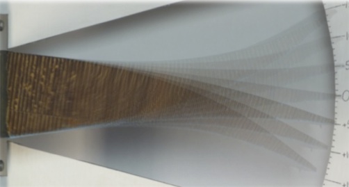
Researchers were having a tough time figuring out why drag increased and lift decreased as an aircraft approached the speed of sound. It was not until 1934 that a young Langley researcher John Stack captured the culprit on a photograph of a high-speed wind tunnel test of an airfoil.
As the aircraft airspeed approaches the speed of sound, small pockets of supersonic flow develop on the suction surface of the airfoil as the airflow accelerates over the curved profile. For thermodynamic reasons these pockets of supersonic flow terminate in normal shock waves and the ensuing increase in pressure exacerbates the adverse pressure gradient on the suction surface. Ultimately, this leads to premature boundary layer separation and thereby decreases lift and increases drag (see figure below). John Stack was the first person to capture this phenomenon on film and paved the way for supersonic flight in the years to come.
Transonic shock wave [6]Other major accomplishments of NASA Langley Research Center include:
The idea of designing specific research aircraft dedicated to supersonic flight, which led to the world’s first transonic wind tunnel
Simulation and testing of landing in lunar gravity using the Lunar Landing Facility
The Viking program for Mars exploration
5 Collier trophies, the U.S. aviation’s more prestigious award, including the 1946 trophy to Lewis A. Rodert, Lawrence D. Bell and a certain Chuck Yeager for the development of a wing deicing system. Fred Welck won the trophy in 1929 for the NACA cowling, an engine cover for drag reduction and improved engine cooling
The grooving of aircraft runways to improve the grip of aircraft tires by reducing aquaplaning, now an international standard for all runways around the world.
Grooved airport runway [7]On March 3rd the NASA reached a major milestone by celebrating its centennial. Since 1917 Langley Research Center has played an important role in the successes of American and international air and space travel. In recent years the media has focused mostly on new commercial space companies such as Orbital Sciences and Space-X.
But as Elon Musk rightly points out, Space X’s exploits would not be possible without NASA’s achievements throughout the last 100 years and its continuing support of the private sector. In fact, NASA made one of it’s first steps into public-private partnerships as early as the 1940’s with the development of the Bell X-1, the first manned aircraft to break the sound barrier.
In that respect join me in congratulating NASA to its centennial and to more exciting aerospace developments for the next 100 years!
References
[1] “Nasa langley test gantry” by Unknown – NASA. Licensed under Public Domain via Wikimedia Commons – https://commons.wikimedia.org/wiki/File:Nasa_langley_test_gantry.jpg#/media/File:Nasa_langley_test_gantry.jpg
[3] “Full Scale Wind Tunnel (NASA Langley)” by Photocopy of photograph (original in the Langley Research Center Archives, Hampton, VA [LaRC]) (L73-5028). Licensed under Public Domain via Wikimedia Commons – https://commons.wikimedia.org/wiki/File:Full_Scale_Wind_Tunnel_(NASA_Langley).jpg#/media/File:Full_Scale_Wind_Tunnel_(NASA_Langley).jpg
[5] “14×22 Subsonic Tunnel NASA Langley” by Erik Axdahl Axda0002. Licensed under CC BY-SA 2.5 via Wikimedia Commons – https://commons.wikimedia.org/wiki/File:14x22_Subsonic_Tunnel_NASA_Langley.jpg#/media/File:14x22_Subsonic_Tunnel_NASA_Langley.jpg
[6] “Transonic flow patterns” by U.S. Federal Aviation Administration – Airplane Flying Handbook. U.S. Government Printing Office, Washington D.C.: U.S. Federal Aviation Administration, p. 15-7. FAA-8083-3A.. Licensed under Public Domain via Wikimedia Commons – https://commons.wikimedia.org/wiki/File:Transonic_flow_patterns.svg#/media/File:Transonic_flow_patterns.svg
[7] “Pista Congonhas03” by Valter Campanato/ABr – Agência Brasil. Licensed under CC BY 3.0 br via Wikimedia Commons – https://commons.wikimedia.org/wiki/File:Pista_Congonhas03.jpg#/media/File:Pista_Congonhas03.jpg
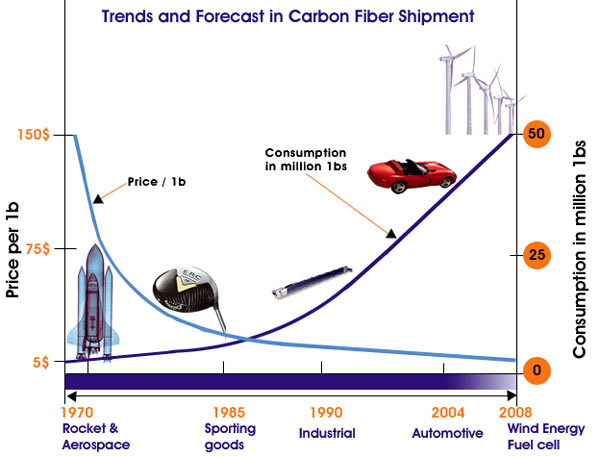
In previous posts I have discussed the unique characteristics and manufacturing processes of a certain type of composite material, namely continuous fibre-reinforced plastics (FRPs). Just like many other composite materials, FRPs combine two or more materials whose combined properties are superior (in a practical engineering sense) to the properties of the constituent materials on their own. What distinguishes FRPs from other composites such as short-fibre composites, nanocomposites or discrete particle composites are the highly aligned, long bundles of fibres typically glass or carbon that are arranged in a specific direction within some resin system.
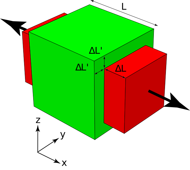
The biggest advantage of FRPs compared to metals is not necessarily their greater specific strength and stiffness (i.e. strength/density and stiffness/density) but the increased design freedom to tailor the structural behaviour. Metals and ceramics, being isotropic materials, behave in an intuitive way since the majority of the coupling terms in the stiffness tensor vanish. If you a imagine a three-dimensional cube and pull two opposing faces apart then the other two pairs of opposing faces will move towards each other. This phenomenon of coupling between tension and compression is known as the Poisson’s effect and aptly captured by the Poisson’s ratio.
The Poisson’s effect in action
In bending, a similar phenomenon occurs known as anti-clastic curvature. If you have ever tried bending a thin, beam-like structure made out of a soft material e.g. a rubber eraser, you might have noticed that the beam wants to develop opposite curvature in the transverse direction to the main bending axis. The structure morphs into some form of saddle shape as shown in the figure. The phenomenon occurs because the bending moment applied by the person in the picture causes tension in the top surface and compression in the bottom surface in the direction of applied bending. From the Poisson’s effect we know that this induces compression in the top surface and tension in the bottom surface in the transverse direction. By analogy, this is exactly the reverse of the bending moment applied by the hands and so the panel bends in the opposite sense in the transverse direction.
Anticlastic curvature in action (1)
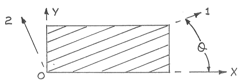
For isotropic materials the fundamental linear constitutive equations between stress and strain eliminate a lot of the possible coupling behaviour. There is no coupling between applied bending moments and twisting. No coupling between stretching/compressing and bending/twisting. And also no coupling between stretching/compressing and shearing. FRPs, being orthotropic materials, i.e. having two orthogonal axes of different material properties, can display all of these effects. Consider a single layer of a continuous fibre-reinforced composite in the figure below. The material axes 1-2 denote the stiffer fibre in the 1-direction and the weaker resin in the 2-direction. If we align the fibres with the global x-axis and apply a load in the x-direction, the layer will stretch/compress along the fibres and compress/stretch in the resin direction in the same way as described previously for isotropic materials. However, if the fibres are aligned at an angle to the x-direction say 45°, and a load is applied in the x-direction then the layer will not only stretch/compress in the x-direction and compress/stretch in the y-direction but also shear. This is because the layer will stretch/compress less in the fibre direction than in the resin direction. This effect can be precluded if the number of +45° layers is balanced by an equal amount of -45° layers stacked on top of each other to form a laminate, e.g. a [45,-45,-45,45] laminate. However, this [45,-45,-45,45] laminate will exhibit bend-twist coupling because the 45° layers are placed further away from the mid plane than the the -45° layers. The bending stiffness of a layer is a factor of the layer thickness cubed and the distance from the axis of bending (here the mid plane) squared. Thus, the outer 45° layers contribute more to the bending stiffness of the laminate than the -45° layers such that the coupling effects do not cancel.
A single fibre reinforced plastic layer with material and global coordinate systems
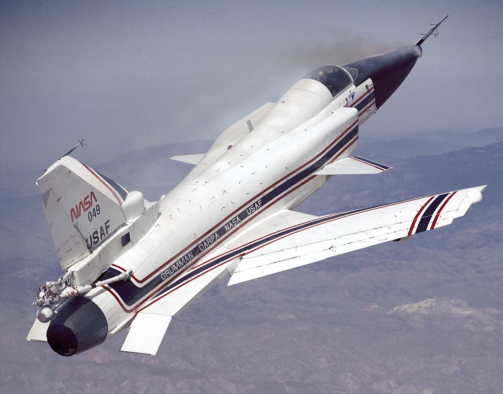
Using metals, structural designers were constrained to tailoring the shape of a structure to optimise its performance i.e. thickness, length and width, and overall profile/shape. FRPs however add an extra dimension for optimisation by allowing designers to tailor the properties through the thickness and thereby achieve all kinds of interesting effects. For example, forward-swept wings on aircraft have and still are a nightmare due to aeroelastic instabilities like flutter and divergence. Basically, sweeping a wing forward is a neat idea because the airflow over swept wings flows spanwise towards the end furthest to the rear of the plane. Therefore, the tip-stall condition characteristic of backward-swept wings is moved towards the fuselage where it can be controlled more effectively. The drawback is that as the lift force bends the wingtip upwards the angle of attack increases, further increasing the lift and thereby causing more bending, and so on until the wings snap off or fail. Rather than adding more material to the wing to make it stiffer (but also heavier) an alternative solution is to use the bend-twist coupling capability of composite laminates. This was successfully achieved in the iconic Grumman X-29. As the bending loads force the wing tips to bend upward and twist the wing to higher angles of attack, the inherent bend-twist coupling of the composite laminate used forces the wing to twist in the opposite direction and thereby counters an increase in the angle of attack. This is an excellent example of an efficient, autonomous and passively activated control system to prevent divergence failure.
Grumman X-29 with forward-swept wings
In this manner, straight fibre composites allow structural engineers to change the stiffness and strength properties through the thickness in order to tailor the structural behaviour. The concept of variable stiffness composites adds a further dimension to the capability for tailoring. Currently this is achieved by spatially varying the point wise fiber orientations by actively steering individual fibre tows using automatic fibre placement machines. One early application that was considered by researchers was improving the stress concentrations around holes by steering fibres around them.
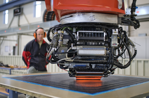
Automated Fibre Placement machine (2)
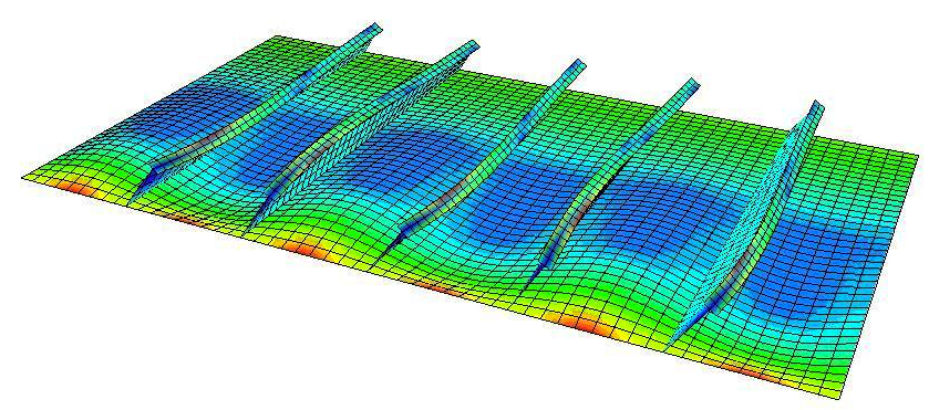
This concept can be generalised by aligning fibres with the direction of local primary load paths which could vary across different parts of the structure. Tow steering creates the possibility for designing blended structures by facilitating smooth transitions between areas with different layup requirements. One promising application of variable stiffness composites is in buckling and postbuckling optimisation of flat and curved panels. As a panel is compressed uni-axially the capability of the panel to resist transverse bending loads reduces until a critical level is reached where the panel has lost all capability to sustain any bending loads. At this point known as the buckling load, the fundamental state of compression becomes unstable and the panel buckles outward in a single or multiple waves. It has been found that variable stiffness composites can double the buckling load of flat panels by favourably redistributing the load paths in the fundamental, pre-buckling compression state. Essentially, the middle of the panel where the buckling waves will occur is offloaded, and the edges of the panel are forced to take more load. Thus, the aim is to redirect loads to locally supported regions and remove load from regions remote from supported boundaries. This concept has also been extended to improving aircraft fuselage sections and blade-stiffened panels.
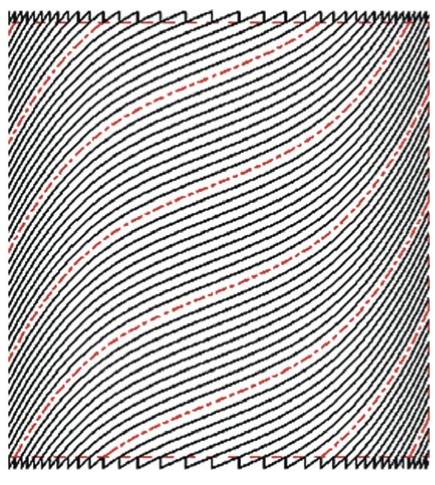
A variable angle tow laminate (3)
This new technology is viewed as a promising candidate for further reducing the mass of future aerospace structures. In fact recently NASA Langley Research Centre announced that they are investing heavily in this capability. The possibility of manufacturing integrated structures with smooth flow of material between components and minimal joints will not only revolutionise stress-based design, but also simplify manufacturing and facilitate entirely new aircraft designs that are currently unfeasible. In trees for example, there is a smooth transition of fibres from the trunk into the branches to strengthen the connecting joint. With the variable stiffness capabilities investigated by NASA we could apply this concept to simplify and even strengthen critical interfaces such as fuselage-wing connections.
Nassim Nicholas Taleb coined the term “Antifragility” in his book of the same name. Antifragility describes objects that gain from random perturbations, i.e. disorder. Taleb writes,
Some things benefit from shocks; they thrive and grow when exposed to volatility, randomness, disorder, and stressors and love adventure , risk, and uncertainty. Yet, in spite of the ubiquity of the phenomenon, there is no word for the exact opposite of fragile. Let us call it antifragile. Antifragility is beyond resilience or robustness. The resilient resists shocks and stays the same; the antifragile gets better. This property is behind everything that has changed with time: evolution, culture, ideas, revolutions, political systems, technological innovation, cultural and economic success, corporate survival, good recipes (say, chicken soup or steak tartare with a drop of cognac), the rise of cities, cultures, legal systems, equatorial forests, bacterial resistance … even our own existence as a species on this planet. And antifragility determines the boundary between what is living and organic (or complex), say, the human body, and what is inert, say, a physical object like the stapler on your desk.
In greek mythology the sword of Damocles is an example of a fragile object as a single large blow will break it, a phoenix can resurrect and is therefore robust, while the Hydra is an antifragile serpent because for every head that is chopped off, two will grow back in its place. Antifragile systems are extremely important in complex environments where black swan events can wreak havoc. Black swans are rare but highly consequential events; the “fat tails” located far away from the mean in a probability distribution.
Often black swan events happen due to non-linear behaviour or a confluence of multiple drivers. Non-linearity is inherently difficult for our brains to comprehend which makes black swan events basically impossible to predict beforehand. In structural mechanics for example, it took researchers years to realise that the buckling behaviour of cylindrical shells, such as fuselage sections, is an inherently non-linear structural phenomenon, and that linear eigenvalue solutions could result in drastic over-predictions of the load carrying capacity. Theodore von Kármán managed to explain the physics of the problem through a series of papers in the first half of the 20th century, by first qualitatively investigating the phenomenon using simple experiments and then formalising the theory in what are now the non-linear von Kármán equations.
But what does this have to do with the engineering design process?
Well, by nature the design process is iterative. Ideally we strive towards creating a system of concurrent engineering. Tasks performed by the design, structural and manufacturing engineers are parallelised and integrated to reduce the development time to market, and reach the best compromise between different technical and financial requirements. Despite this parallelisation, the design process within each of these departments is still highly iterative as engineers across different functional fields interact and refine the design. Most importantly, throughout the whole aircraft design process individual components and sub-assemblies are experimentally tested to verify the design under critical load conditions. Examples of these are cabin section pressurisation fatigue tests and catastrophic tests of whole wing sub-assemblies. The information of these stress tests is fed back into the design system to close the loop and inform the next stage in the design.
Design Cycle Structural Engineering
Taleb calls this form innovative work “stochastic tinkering”. It is a means of experimenting and adjusting a system, aiming to discover fact “A” but in the process also learning about “B”. Stochastic tinkering is by nature antifragile as good aspects of a design are retained while failures are quickly removed; very much an analog of the evolutionary process in nature.
Of course there is a good deal of deterministic analysis involved in engineering design. However, preliminary design calculations are often based on “back-of-the-envelope” methods. The aim of these preliminary calculations is to constrain the design space to a smaller feasible region. The design is then refined further in the detail design stage using more advanced techniques such as Finite Element Analysis or Computational Fluid Mechanics. Crucially, no matter how beautiful the design works on paper if it doesn’t perform in the validation tests it has failed.
Finally, the notion of designing for black swan events is inherently incorporated in the design process. In structural analysis of aircraft hundreds of different load cases are tested individually and in confluence to make sure the structure can withstand the worst imaginable/historic loading scenario multiplied by a factor of safety. Furthermore, the “safe-life”, “fail-safe” and “damage tolerant” design frameworks create a checklist for components which:
are absolutely not allowed to fail during service (e.g. landing gear and wing root)
are allowed to fail, as structural redundancies are in place to re-direct load paths (e.g. wing stringers and engines)
and components that are assumed to contain a finite initial defect size before entering service that may grow due to fatigue loading in-service. In this manner the aircraft structure is designed to sustain structural damage without compromising safety up to a critical damage size that can be easily detected by visual inspection between flights.
This approach is limited to known load cases. Therefore, the reserve factors of 1.2 for limit load and 1.5 for ultimate load exist to provide a margin of safety against uncertainty, i.e. things we can not quantify, the “known unknowns” and “unknown unknowns”.
Historically, catastrophic in-service failures have been and continue to be used as invaluable learning experiences. Thus, “fat tail” catastrophic events are continually being used to eradicate weaknesses and improve the design. This, in essence, is the definition of antifragility. As terrible as the loss of life in the DeHavilland Comet and other crashes have been, without them, airplane travel would not be as safe as it is today.
Understanding the details of the atmosphere is critical for manned flight since it provides the medium through which the aircraft moves. The lift provided by the wings and drag experienced by the aircraft vary greatly with different altitudes. In fact Sir Frank Whittle was largely motivated to design a jet engine due to his insight that aircraft would be able to fly faster and more efficiently at higher altitudes due to the lower density of air. The internal combustion engines at the time would not allow higher altitudes of flight, since the lack of oxygen was starving the engines thereby reducing power output.
In essence the atmosphere is a fluid skin that surrounds the entire earth to around 500 miles above the surface. Measured by volume the atmosphere at sea level is composed of 78% nitrogen, 20.9% oxygen, 0.9% Argon, 0.03% Carbon Dioxide and a trace of other gases. Up to about 50 miles the composition of the air is fairly constant, except for a variation in water vapour, which depends on the ambient temperature. The hotter the air the more water vapour it can hold (this is why you can see your breath on a cold morning as the cold air is saturated at this lower temperature). The heavier gases do not rise to high altitudes such that above 50 miles the atmosphere is largely comprised of hydrogen and helium. Above 18 000ft oxygen has depleted enough to prevent human’s from breathing and so oxygen is supplied mechanically to the cabin. At about 100 000ft oxygen is too low to allow combustion even in the most advanced turbojet engines.
In lower temperature latitudes the 36 000 ft of the atmosphere are generally known as the troposphere. In the troposphere the temperature decreases from about 20°C at sea level to -53°C. The tropopause is a hypothetical boundary between the lower troposphere and the higher stratosphere. In the stratosphere the temperature is initially constant and then increases to about -20°C at 35 miles. The separating tropopause is not a clear cut line but rather a hypothetical boundary that varies from around 30 000 ft over the poles to around 54 000 ft above the equator. As a result the temperature in the stratosphere is naturally warmer over the poles than over the tropics, since the higher altitude of the tropopause over the tropics allows the temperature to fall further before the constant temperature region of the stratosphere is reached. The atmosphere is divided further into regions such as the mesosphere, mesopause, thermosphere and the exosphere. However, these regions are outside of the realms of commercial and most fighter aircraft and we will therefore not deal with them here.
As originally observed by Sir Frank Whittle, the atmospheric conditions have a great effect on the performance of aircraft:
The local ambient conditions of the air influence lift, drag and engine performance. In particular the pressure, density and temperature of the local air define the performance characteristics.
The aircraft is moving relative to a fluid mass that in turn is moving relative to the surface of the earth. This introduces navigational problems that require special on-board equipment to control flight speed and direction.
Temperature variations within the atmosphere may cause adverse weather patterns such as strong winds, turbulence, thunderstorms, heavy rain, snow, hail or fog. These criteria influence the loads applied on the aircraft, safety and the comfort of the passengers.
The presence of the chemical compound ozone at high altitudes prevents cabin pressurisation with ambient air. This present the designer additional problems with air conditioning and prevention against pressure-cabin failure.
Air is a compressible fluid (i.e. it can change in volume and pressure in contrast to fluids which are largely incompressible). The compressibility of air allows it change shape and shear (flow) under the smallest pressure changes. The relation between pressure p, temperature T and volume v is governed by the ideal gas equation:
[latex] pv = RT [/latex]
where R is the universal gas constant 287.07 J/kg/K and temperature is measured in Kelvin (T in °C + 273). In order to standardise calculations relating to the atmosphere the International Civil Aviation Organization has chosen a definition of the “standard atmosphere”. This states that air is a perfectly dry gas with a temperature at sea level of 15°C and 101.3 kPa of pressure. For the first 11 000km (i.e. in the troposphere) the temperature is assumed to change at a constant lapse rate of -6.5 °C/km, then stays constant at -56.5°C in the troposphere (11 000- 20 000 km) and then increases at different rates in the stratosphere. Another important metric for aircraft flight is the dynamic viscosity of “stickiness” of the air, which influences the drag imposed on the aircraft. You can imagine air being composed of thin layers of air that move relative to each other similar to multiple pieces of paper in a notebook. The dynamic viscosity is the constant of proportionality between the force per unit area required to shear the different sheets over each other and the velocity gradient between the layers. At ordinary pressures the dynamic viscosity generally depends only on the temperature of the air.
Finally the local atmospheric conditions is why aircraft engineers and pilots differentiate between the quantities of true airspeed (TAS), which is measured relative to the undisturbed air, and a fictional speed called the equivalent airspeed (EAS). The latter is of prime importance for aircraft design since it defines the forces that are acting on the aircraft. TAS and EAS are equivalent at sea level in the standard atmosphere but vary at altitude. As an aircraft moves through a mass of initially stationary air it imparts momentum to the surrounding air molecules by both impact and friction. The first molecules that hit the aircraft can be imagined to stick to the aircraft surface and are therefore stationary with respect to the aircraft. Every unit volume of air that has been accelerated to the velocity of the aircraft V, has therefore been imparted with a kinetic energy of
[latex]q = \frac{1}{2} \rho V^2[/latex]
where q is known as the dynamic pressure. Aerodynamic quantities such as lift and drag are typically expressed as non-dimensional parameters i.e. they are divided by the wing area and the dynamic pressure to give the lift coefficient and drag coefficient.
[latex]C_L= \frac{Lift}{qS}, [/latex]
[latex]C_D= \frac{Drag}{qS} [/latex]
The non-dimensional form of the parameters is important since it allows a performance comparison between different wings operating at different flying speeds or density conditions. Thus for an aircraft with a specific lift coefficient and wing area to generate the same aerodynamic forces at altitude as at sea level, the aircraft must be flown at a velocity that keeps the dynamic pressure a constant, regardless of any difference in air density. Thus, if the density at flying altitude is [latex]\rho[/latex] and the airspeed measured by the onboard controls is the TAS, then the equivalent speed at sea-level EAS with density [latex]\rho_0[/latex] is defined by,
[latex]EAS = TAS \sqrt{\frac{\rho}{\rho_0}}[/latex]
Therefore the EAS is a fictional quantity used in aerodynamic calculations to defined the speed that gives the same aerodynamic forces at sea-level as those experienced at altitude.
I have just returned from the International Conference for Composite Materials (ICCM) in Montreal, Canada and would like to share a few observations and key points about the developments in the composite world that may not be so easily accessible to a broader audience.
1) The Great Advance – Applications
ICCM is the biggest conference for composite materials and this year united over 1500 delegates from academia and different industrial representatives from the classical sectors aerospace, wind energy and high performance cars to newer sectors such as mass market cars (e.g. BMW i3), biomedical applications and even musical instruments. The motto of the conference “Composite Materials: The Great Advance” aptly captures the current state of technology in the industry. Since the 1960 considerable amount of research has been conducted to elucidate the mechanical and chemical properties of the fibre material, matrix and cured composite under various conditions such that the global behaviour of these materials is now sufficiently characterised. This maturity in technology coupled with the ever decreasing costs and the inherent benefits of high specific stiffness and strength that fibre-reinforced plastics have to offer, has led to the increasing application of composite materials in very different industries that we see today. Thus the “great advance” of composite materials towards wide-spread use in many industrial sectors.
Fig. 1. Composite materials growth broken down by sectors (1)
Fig. 2. Carbon Fibre Market (2)
2) The Great Advance – Novel Technologies
Furthermore, “The Great Advance” also relates to novel composite materials with much greater complexity that blur the lines between what is a material and what is a structure. Of course on a macroscopic scale one could say the steel in a steel bridge is the “material” that has been used to construct the “structure” that is the bridge. Therefore in this classical interpretation steel is just the building block to make the bridge, while the structure itself is the final product that performs a function. However on a microscopic scale we could argue that steel is a structure in itself since it is “constructed” of different sized grains that contain different metallic compounds and is thus an arrangement of small particles i.e. a microstructure. We could of course continue this argument further and further up to the atomic scale at which point we have reached the field of nanotechnology. This field of research has enjoyed much popularity in recent years since by manufacturing our products from the ground-up, i.e. from the nanoscale to the macroscale, we can control the properties of our product at multiple length-scales and therefore tailor the characteristics to be optimal for the desired function in service or even add some sort of multi-functionality to the structure/material. Since the material and structure are built at the same time the dividing line that used to distinguish between these two concepts is blurred. Even for a simple composite laminate comprised of a stack of individual layers this divide is no longer so clear since we can define the properties of each ply in the stacking direction and therefore have control over one more length scale.
Therefore in the future there will be a great advance towards novel and multifunctional materials/structures that perform so much more than carrying structural loads. Currently the design of composite structures is still in some cases dominated by a “black aluminium” approach. That is taking the current designs that have worked so well over the last decades using aluminium and replacing them by an equivalent composite design. The problem with this is that on one hand the composite material may not be suitable to carry loads in the same configuration e.g. loads through the thickness have to be avoided to prevent delaminations. Most importantly however, such a design approach hinders the greatest advantage of this new material system, which is to facilitate entirely new structures in terms of functionality and shape that arise as a results of their inherent properties. Only by completely re-designing structures from the ground-up and taking the intricacies of this new material system into consideration can we arrive a new optimal solutions or conversely ascertain that a metal solution actually works better under some circumstances. In the following I want to share a few exciting technologies that you may see in the near future.
1) Variable stiffness technology
This is my field of research and essentially what we are currently doing is changing the fibre direction over the planform of the plate such that we have curvilinear fibres rather than the straight fibre laminates that we use today. In many aerospace applications we require different laminate stacking sequences in different parts of the structure. Abruptly changing from one stacking sequence to another can lead to stress concentrations and thus structurally weaker areas at the interface. Using the variable fibre concept we can easily spatially blend from one layup to another to reduce these problems. Furthermore, we can arrange the fibre paths to follow the dominant load paths as for example around a window in an aircraft fuselage. Loads in a structure always follow the path of highest stiffness. So by aligning the fibres in the load direction in supported areas of the laminate (for example the vertical edges in Fig. 3 below if the load is applied vertically onto the horizontal edges), a large portion of the stress can be removed from the unsupported centre of the panel, which can greatly improve the elastic stability of the structure. This has great potential for future wing structures since the design of wing skins is greatly governed by local buckling (Fig. 4). It has been shown that the buckling loads can be improved by 70%-100% using variable stiffness technology (5), thus the possibility exists to reduce the weight of wing structures by up to 20% using this technology.
Fig. 3. A variable angle tow laminates (3)
Fig. 4. Buckling analysis of a stiffened wing panel. The stiffeners break the buckling mode shapes into smaller wavelengths that require higher energy to form than a single wave (4)
Another form of various stiffness technology is placing material in areas where it is needed and removing it from areas where it is not required. Nature is an expert in achieving this and many of our current design are based on bio-mimicry. For example, your bones are continuously being re-modelled based on the stresses that are placed on your skeleton. In this way the density of your bones is increased in highly-stresses areas and decreased in areas that are not used so much. In the same way sea-sponge arranges its structure in a way to achieve the most efficient design. Similarly, wood possesses an incredibly complex microstructure that is composed of different structural hierarchies at different length scales. This is similar to a rope where individual fibres are twisted together to make strands, strands are twisted together to make bundles, and bundles twisted together to make the complete rope. This approach of designing at multiple length-scales makes wood very ductile and resilient to cracks. In this manner attempts have been made to reproduce such a hierarchical design by arranging short fibres using standing ultrasonic waves.
Fig. 5. Microstructure of wood. Notice the different structures at different length scales that gives wood its inherent strength (6).
2) Self Healing
Yes, materials can heal themselves. The most popular example is that of self-healing asphalt, which was presented a few years ago at a TED conference. In terms of composites 100% recuperation of mechanical properties have been achieved when the mode of failure has been dominated by matrix cracks. In high performance composites the matrix is currently some sort of thermoset or thermoplastic, which allows vascules of uncured resin to be included in the structure which may break open as a crack propagates. The uncured resin then permeates through the open crack and cures in-situ to repair the full functionality of the part. The dissemination of the healing process can also be achieved using very thin vascules that are arranged throughout the part. In this manner the structure starts to behave very much like a living organisms with the vascules serving as pathways for repair very similar to the veins in an organism. Recently, a great article by the BBC summarised the major achievements in this field.
Fig. 6. Self healing capsules (7)
Fig. 7. Self healing vascules (7)
3) Nanotechnology
Nanotechnology has been extremely popular during the last 20 years due to the fact that theoretical predictions promise incredible benefits for almost all applications in engineering. In terms of advanced composites however, there are still problems of evenly dispersing nanotubes in resins with agglomeration or alternatively producing continuous nano-strands at low costs. In the aerospace industry they show great promise in increasing the electrical conductivity of laminates to improve their resistance against lightning-strike, creating structures for magnetic shielding and providing interlaminar strengthening using nano-forests. One of the cooler things I saw at ICCM was research conducted on nano-muscles, which are essentially nano-fibres that have been twisted into a rope and can achieve very high actuation forces and strokes at very little mass.
4) Structural Batteries / Energy Harvesting
Solar power has incredible potential as an energy source since it is the largest form of energy available for consumption on earth and is limitless. However, solar power is sporadically dependent on the weather conditions, which makes energy conversion rather cost intensive and inefficient. However, solar energy harvesting might find increasing use if actively integrated into load-bearing components as a multi-functional structure. Bonding thin-film solar cells onto lightweight composites would eliminate the material redundancy of stand-alone supporting structures and could easily be integrated into current laminate manufacturing technology. Photovoltaic (PV) cells have been embedded in composite laminates and their performance has not been impeded by the curing process. However, the performance of the PV cells diminishes rapidly under static loading since the loading causes cracks in the cells. Similarly there are ideas to create structural batteries such that the load carrying chassis of a car can be “charged-up” to additionally serve as the battery for an electric powertrain. Of course this would have the great advantage that the heavy batteries used today could be eliminated to some extent. BAE systems are working on technology to embed battery chemistries into the carbon fibre fabric.
5) Morphing
Finally, morphing or shape-changing structures have been extensively studied since the 1970’s for providing aircraft with the possibility of adapting the shape of their wings to provide the optimal lift for different flight scenarios. Of course this is to some extent already used in aircraft with the aid of leading edge slats and trailing-edge flaps to increase the lift-coefficient for slower flight regimes such as landing and lift-off and in Formula 1 using drag reduction system of the rear wing. However, slats and flaps on an aircraft greatly increase the drag of the profile during deployment and increase the weight of the structure do the heavy actuation mechanism. Therefore the aim is to design an integral system such as the trailing-edge design shown below. Other examples of morphing structures include air intakes for cars, noise-reducing chevrons on jet-engines, or high-temperature composites used for jet-engine turbine blades that change there angle of attack based on the temperature of the airflow around them.
Fig. 8. A morphing trailing edge using a flexible honeycomb (8).
However, in most cases these technologies are very difficult to apply to primary aircraft structures. This is because there is a direct conflict between the high-stiffness, high-strength requirement for carrying loads and the low-stiffness, large-deflections required for shape-changes. Thus, a driver to facilitate these technologies will be the development of materials that change there mechanical properties under different circumstances.
3) The Great Advance – Solving “big” problems for larger scale implementation
Finally, one of themes during the conference was trying to solve some of the major problems faced by the industry hindering further implementation of current composite technology in all industrial sectors. Of course for some industries such as mass consumer automobiles the biggest barrier to entry is cost. The new BMW i3, which will enter the marketplace at the start of 2014, will cost £30,000+ and is therefore quite a big investment for a small city vehicle. Of course some of the cost can be attributed to the cost of the electrical drivetrain and batteries but other manufacturers such as Renault have shown that a lot of these costs can be reduced by employing a scheme based on renting batteries rather than buying them with the vehicle. In case of the i3 a lot of the extra cost is simply down to the fact that BMW are the first to build a mass produced automobile using a large amount of fibre-reinforced plastics in primary structural parts. Not only is cost of raw material much higher than for lightweight metals such as aluminium but the manufacturing processes and supply chain management required for reliable mass production were simply not in-place beforehand. Furthermore, a shift in design methodologies is required since the chemical and mechanical behaviour of composites is so different from the metal environment that the automobile industry is so used to dealing with. As an example, proving the structural integrity for the incredible rigorous crash/impact certification using rather brittle composite materials compared to more ductile metals is a challenge in itself. Thus, the relatively high price-tag of the i3 incorporates some of the research and development costs that BMW have had to face in developing composite technology for their market sector. No doubt the cost of mass market composite cars will reduce drastically in the next decade as the raw material price further reduces and design methodologies and manufacturing processes mature.
Another major issue hindering the implementation of composites especially in the aerospace industry is the difficulty of predicting the failure behaviour of these materials. On problem is the large number of failure modes that may occur: fibre breakage, matrix cracks, delamination, fibre crimping, fibre-matrix debonding, global and local buckling etc. and thus finding accurate failure loads for all these phenomena under different load cases. Since a larger number of these failure mechanisms originate on a local, micro-mechanical scale high-fidelity 3D Finite Element models are often needed to fully understand the mechanisms of failure and predict the load-carrying capability of different structures. Considering the size of any commercial aircraft it is absolutely inconceivable to apply such detailed and computationally expensive analysis tools to every part of an aircraft. Furthermore, the failure mechanisms are not as well defined as for metal materials. That is in classical tensile or compressive tests a specimen may undergo some form of non-linearity that may for a metal specimen be classified as a failure event but for the composite considerable residual strength is available. Conversely the failure behaviour of composites can be very brittle with very little warning compared to the gradual, ductile failure mechanism of most metals used in the aerospace industry. Considering the intricacies of composite failure modes and the fact that the individual failure modes may interact or even change in criticality depending on the size of the component and environment in which it is used, it is no wonder that currently very conservative safety factors are being employed for primary composite aircraft structures that greatly offset the weight-savings that are possible using this new material system. Thus, one of the biggest if not the biggest topic in composite structural design for the next couple of years will be the challenge of developing simple and yet robust failure criteria to be used for composite designers.
(5) Gürdal Z, Tatting B, Wu C. (2008). “Variable stiffness composite panels: Effects of stiffness variation on the in-plane and buckling response”. Composites: Part A, 39(5), pp. 911-922.
(6) Greil P, Lifka T, Kaindl, A. (1998). “Biomorphic Cellular Silicon Carbide Ceramics from Wood: I. Processing and Microstructure”. Journal of European Ceramic Society, 18(14), pp. 1961-1973.
(7) Rincon, P. (2012). “Time to heal: The material that heal themselves.”http://www.bbc.co.uk/news/science-environment-19781862
(8) Daynes S & Weaver P.M. (2011). “A Morphing Wind Turbine Blade Control Surface”. Proceedings of the ASME 2011 Conference on Smart Materials, Adaptive Structures and Intelligent Systems. Phoenix, AZ: ASME.

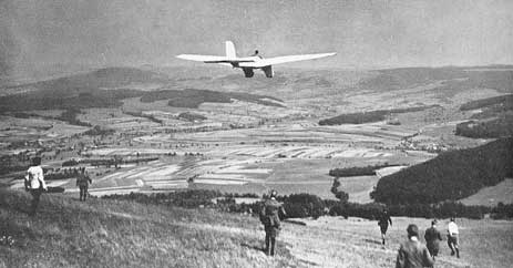

.jpg)
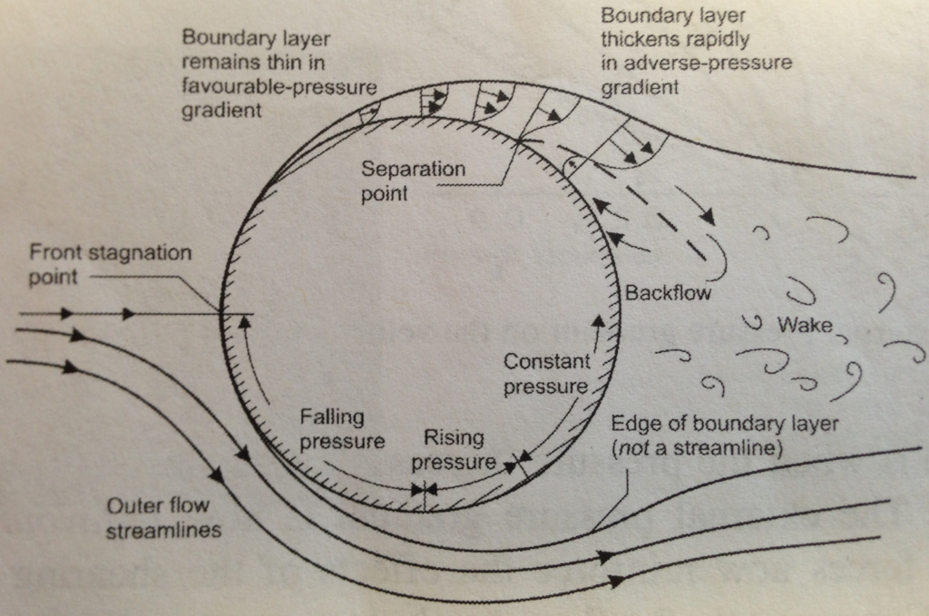


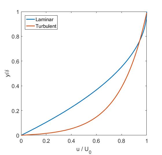
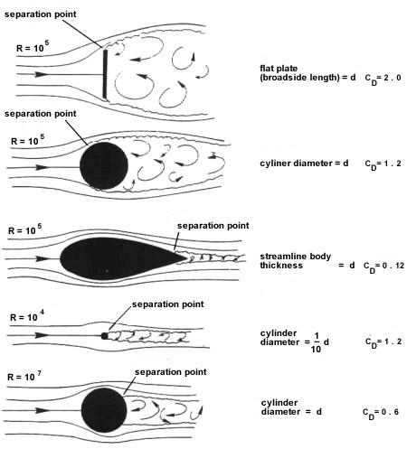


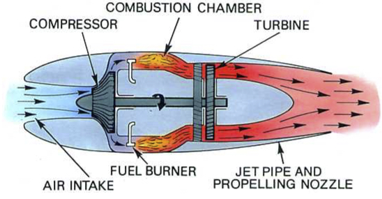
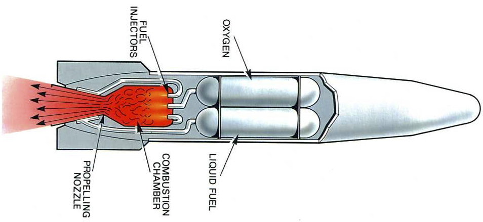
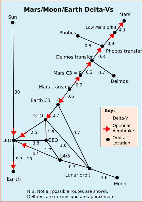
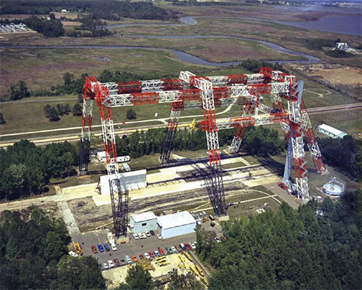
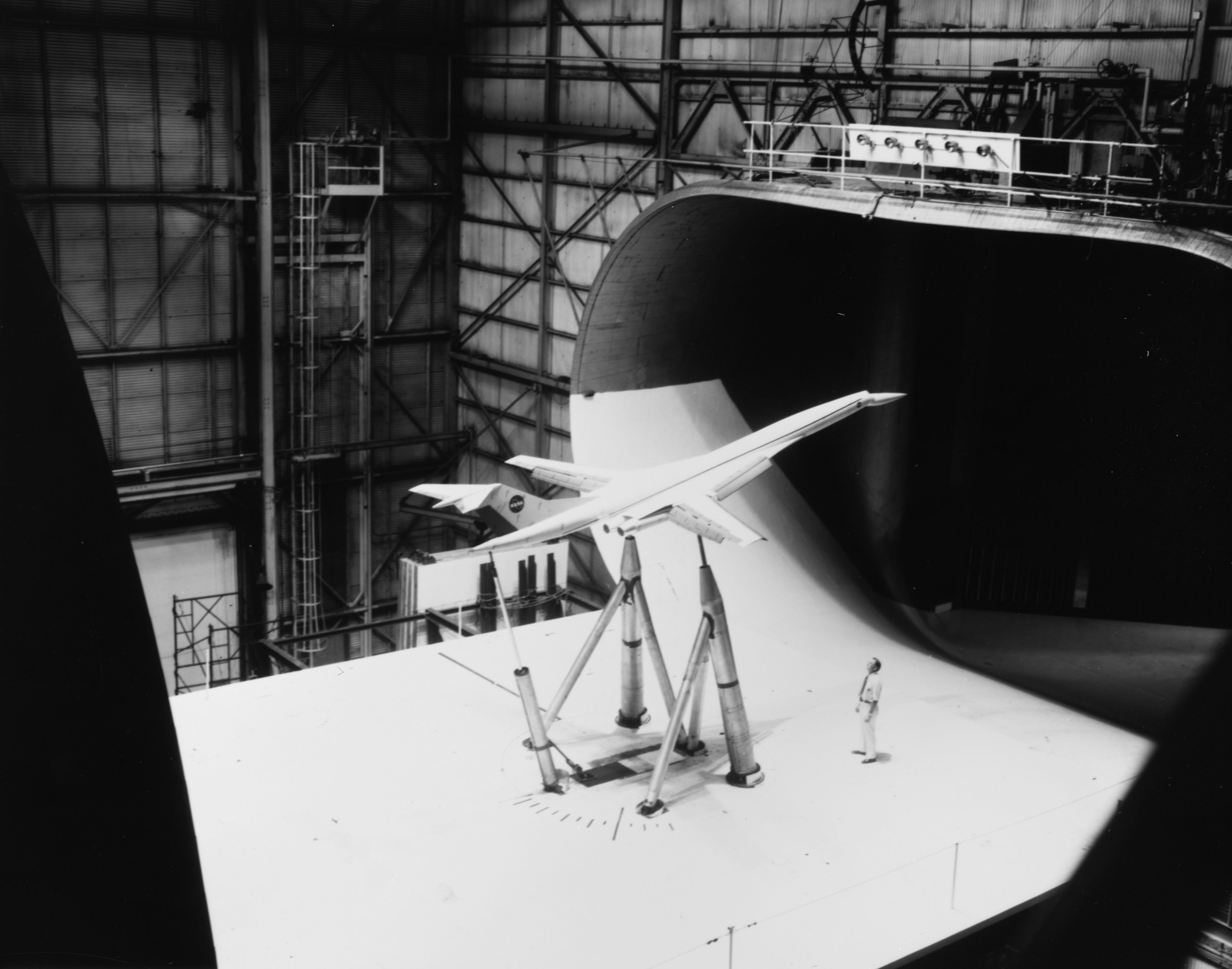
![NASA Langley subsonic wind tunnel [2]](https://rgroh.com/wp-content/uploads/2015/05/14x22_Subsonic_Tunnel_NASA_Langley.jpg)
![Transonic shock wave [4]](https://rgroh.com/wp-content/uploads/2015/05/Transonic_flow_patterns.svg_.png)
![Grooved airport runway [3]](https://rgroh.com/wp-content/uploads/2015/05/Pista_Congonhas03.jpg)