Priyanka Dhopade received her PhD from the University of New South Wales in Canberra, Australia and was the recipient of the Zonta Amelia Earhart Fellowship award, awarded annually to the 35 most outstanding female aerospace PhD students worldwide. Since 2013 she has been researching the thermodynamics of jet engines in the Thermofluids Institute at Oxford University. Priyanka is an expert in computational fluid dynamics modelling of heat transfer, aerodynamics and aero-elasticity in jet engines. She is currently leading the modelling campaigns for various projects in collaboration with industry partners relating to turbine and compressor tip clearance control, turbine internal cooling and active flow control. In this episode, Priyanka and I talk about:
the challenges of improving the efficiency of current gas turbines
the intricacies of fluid dynamics modelling
and a topic particularly close to her heart, the diversity challenge in STEM fields.
This post is a first. Up to now, all content on this blog has been exclusively written by myself. But recently Nick Mehlig and Ben Names from Structural Design and Analysis, Inc. (SDA), a team of stress engineers that design lightweight and load efficient structures, contacted me with a proposal for a guest post. The reason why I agreed is because the guys at SDA have a unique perspective on a fascinating real-world engineering problem — re-designing the wing of a Fokker D-VII. The Fokker D-VII was a German fighter aircraft in World War I but was also used by many other countries after the Great War. This post is a look at some of the details of how aircraft components are designed.
Within the Aerospace Engineering community, there is an entire sub-discipline devoted to understanding the dynamics of a system and how loads are generated (propulsive, inertial, aerodynamic, etc). In smaller companies, engineers often need to wear multiple hats, and the lines between classical stress analysis and aerodynamic loads analysis begin to blur. Recently, Structural Design and Analysis, Inc. (SDA) worked with a local resident who had taken it upon himself to build a Fokker D-VII Biplane from scratch, and wanted to know how much weight he could save if he used an aluminium spar for the main wings instead of the original wooden spar design.
Our engineers had to develop a finite element model (FEM) and conduct the basic loads and dynamics analysis to define the load cases for the vehicle. Generating aerodynamic loads is relatively straight forward for aircraft with more conventional designs. Typically, a combination of 2D aerodynamic theory and corrections for wings with finite span are used to generate the loads in the early stages of the design phase. These loads are then applied to the structure at the quarter chord location of the wing. For the Fokker, this analysis is slightly more complicated because the biplane construction creates interference effects between the upper and lower wing which must be considered when determining the loads that act on the aircraft.
The goal of this case study is to show that various approaches can be taken to solve this loads-generation problem, and that the “best” approach for an engineer depends on his/her technical expertise, available resources (time and/or money), and the desired accuracy of the results. Three different methods were selected to calculate the aerodynamic loading on the Fokker D-VII biplane, and they are listed in increasing order of required technical expertise and accuracy:
Assuming that each wing can be analysed separately. This type of solution is best suited to an aircraft enthusiast or an engineer without much background in theoretical aerodynamics.
Accounting for the interaction between the upper and lower wing using correction factors. This type of solution is best suited for an engineer with a level of understanding comparable to an undergraduate education in aerospace engineering.
Using an advanced FEM analyses suite such as NX Nastran’s Static Aeroelastic SOL 144. This solution technique requires the least amount of effort on the user since the loads are calculated internally by NX Nastran, but is best suited to an engineer with some postgraduate education in aerospace engineering.
Let’s compares the efficacy of these three methods and the accuracy of their respective results.
Method 1
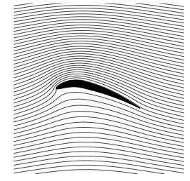
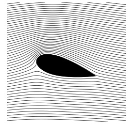
The first step in calculating the aerodynamic loads on the aircraft is to get the airfoil data. The Fokker D-VII uses a modified Goettigen GOE 418 airfoil for the upper wing. The airfoil data points (see the diagram below) were imported into XFOIL, a popular open-source 2D potential flow code, and the lift coefficients were extracted for various angles of attack (AOA). Using the XFOIL data, a plot relating the wing’s AOA to the lift coefficient ([latex] C_L [/latex]) is constructed. A trendline is added to the data to estimate the lift curve slope for the airfoil of [latex] C_{L_\alpha} = 0.095/^\circ [/latex] and the zero lift AOA is [latex]-8^\circ[/latex](the airfoil is angled down for no lift).
To calculate the lift on the upper and lower wings, a simple approximation from Prandtl Lifting Line Theory is used which relates the 3D lift coefficient to the 2D lift curve slope, the wing aspect ratio (AR) and the AOA. The lower wing of the Fokker D-VII has a [latex] 1^\circ [/latex] AOA while the upper wing has [latex] 0^\circ [/latex] AOA.
where [latex] S [/latex] is the wing area and [latex] q = 1/2 \rho V^2 [/latex] is the dynamic pressure that depends on the density [latex] \rho [/latex] and the airspeed [latex] V [/latex] of the particular manoeuvre.
To balance the aircraft, the moment created by the wing lift about the centre of gravity of the Fokker needs to be balanced by the tail wing lift force, [latex] F_{tail}[/latex]. Each moment is equal to the lift force multiplied by the distance of the point of action [latex] x [/latex] from the centre of gravity of the aircraft. Given the relative positions of the two wings and the tail plane, we solve the following equation
The sum of these three loads is [latex] 3,110.73+2,204.19+79.40 = 5,394.32 [/latex] lb or 4.31g’s. Since we are analysing a 4.0g load case here, the lift on the wings will need to be reduced. As the lift on the wings is reduced, the pitching moment will change which, in turn, changes the required tail force to balance the aircraft. Excel’s goal seek was used to reduce the wing loading and balance the aircraft such that the total lift (including the tail) is equal to 4.0g. The final loads are shown below.
[latex] L_{upper} = 2,894.41 [/latex] lb
[latex] L_{lower} = 2,078.78 [/latex] lb
[latex] F_{tail} = 62.81 [/latex] lb
These final loads are applied to the quarter chord location of the wings. Here, a rectangular spanwise lift distribution is applied to the upper and lower wings.
Method 2
By having two wings subject to the same flow, each wing interacts with the other’s vortex system such that the upper wing experiences an increase in lift and the lower wing experiences a decrease in lift, denoted by [latex] \Delta C_{L,upper} [/latex] and [latex] \Delta C_{L,lower} [/latex] respectively. The following method uses the simple biplane theory which is detailed in NACA Technical Report No. 458 [1]. It is shown that the change in lift coefficient [latex] \Delta C_{L} [/latex] follows a linear relation with the overall vehicle lift coefficient [latex] C_{L} [/latex] in the following form:
Where [latex] K_1 [/latex] and [latex] K_2 [/latex] are constants relating to the gap between the two wings, wing stagger (the relative fore-aft position of the two wings), decalage (angle difference between the upper and lower wings of the biplane), overhang (the extension of one wing span over the other), and wing thickness. The change in lift for the lower wing is related to the change in lift of the upper wing by the ratio of wing areas.
The methods of finding the values of [latex] K_1 [/latex] and [latex] K_2 [/latex] follow a graphical approach using the biplane ratios of wing gap = 55 in., wing stagger = 25 in. , percent wing overhang = 17.4%, and decalage = 1 deg. Using these values and the method described in NACA Report 458, the following values are calculated: [latex] K_1 = -0.090 [/latex] and [latex] K_2 = 0.195 [/latex]. The final lift coefficient for the upper and lower wings are found by adding the correction to the vehicle lift coefficient to the original uncorrected value. This uncorrected value is calculated from the maximum weight of the aircraft, which naturally determines the lift required from the wings. The maximum weight of the Fokker D-VII is 1,259 lbs, and for a 4.0g manoeuvre (n=4 in the equation below), the aircraft lift coefficient is:
Plugging in values for [latex] K_1 [/latex], [latex] K_2 [/latex] and [latex] C_L [/latex] into the [latex] \Delta C_{L,upper}[/latex] and [latex] \Delta C_{L,lower}[/latex] equations give the following values:
Using the new corrected values for the wing coefficients [latex] C_{L,upper} = C_L + \Delta C_{L,upper}[/latex] and [latex] C_{L,lower} = C_L + \Delta C_{L,lower}[/latex], the total load can be calculated for the upper and lower wings. A moment balance is performed and the following loads are calculated for the aircraft:
[latex] L_{upper} = 3,139.88 [/latex] lb
[latex] L_{lower} = 1,803.24[/latex] lb
[latex] F_{tail} = 92.87[/latex] lb
Again, the loads are applied to the quarter-chord position of the aircraft wings. Two different spanwise lift distributions are applied to the model for this comparison study. The first assumes an elliptical lift distribution. The second uses Schrenk’s Approximation to estimate a more accurate spanwise lift distribution. These two distributions are shown below along with a reference to a rectangular distribution.
Method 3
The third and final method is to use NX Nastran’s static aeroelastic SOL 144 analysis to generate the loads using a vortex lattice formulation. A potential flow model is created in FEMAP to generate the aerodynamic loading for the Fokker. One of the powerful functionalities about SOL 144 trim analysis is that given high-level information about any flight condition, Nastran cannot only calculate the aerodynamic forces, but can also ensure that the vehicle is stable. With just a few clicks, the load case can be modified to model any corner of the flight envelope by changing the dynamic pressure and load factor of the aircraft. Since Nastran calculates all the loads internally using this high-level flight condition information, it can save an incredible amount of time that might be devoted to calculating loads externally, bringing them in, and applying them to the structure accurately. This solution requires the least amount of effort on the user since the loads are calculated internally by NX Nastran and then applied to the FEM through the points defined in the model. NX Nastran automatically calculates the trim condition of the aircraft and calculates the loading on the upper wing, lower wing, and horizontal tail. The resulting loads are shown below:
[latex] L_{upper} = 3223.21 [/latex] lb
[latex] L_{lower} = 1,697.10[/latex] lb
[latex] F_{tail} = 122.75 [/latex] lb
Results
As the complexity increases with each of the methods discussed above, so does the accuracy of the results. However, not every stage of the design requires the same precision. Since this discussion focuses on how the analysis approach impacts the design of the aircraft, let us first compare the calculated loads for all three methods. Below is a table outlining the loads for each method and the percentage difference when compared to the aeroelasticity finite element model (the most accurate loads generation approach).
When comparing the lifting force of upper and lower wings of the aircraft, the aerodynamic loading from method 1 underestimates the lift on the upper wing by 10.2% and over estimates the lift on the lower wing by 22.5%. Applying Simple Biplane Theory in method 2 captures the interference effects and estimates the wing loading much more accurately with the upper wing lift only 2.6% less and the lower wing lift 6.3% greater, when compared to the aeroelastic model. A more detailed way to compare the resulting design impact of the three different load generation methods is to look at the internal shear and bending moment diagrams within the spars. Below is the shear force diagram for the upper wing leading edge spar.
Starting with the simplest method, the 2D non-interfering lift generates the highest shear force. As one would expect the variation in the maximum internal shear force is small (at most 7% difference) over all the models since the total lift generated by the plane was set to be constant. The differences are partially due to how the lift is distributed between the upper and lower wings. Furthermore, the spanwise distribution clearly has an impact on the internal shear force. Interestingly, the model that matches the shear force of the aeroelasticity model the closest is the Biplane Theory model using Schrenk’s approximation. The differences produced by these aerodynamic models becomes even more apparent when inspecting the internal bending moment.
The internal bending moment clearly shows how differences in the aerodynamic models can propagate. The most basic model (2D Non-interfering Lift) produces the highest bending moment, 33% higher than the aeroelastic solution. While it is safer to be on the conservative side, this kind of inaccuracy will lead to a substantially heavier structure, thus limiting performance.
The shear and bending moment diagrams are often excellent indicators of the internal stress state within simple structures. As a stress engineer, comparing stress plots is the most meaningful way to compare how the different aerodynamics models impact the stress throughout the vehicle. Below is a picture of the upper wing leading and trailing edge spars Von Mises stress under a 4g pull up when using the aeroelasticity model.
The max spar cap Von Mises stress is 11.4 ksi. In comparison, the same stress contour is presented below, only for the case using the Biplane theory using Schrenk’s approximation, which exhibited a maximum Von Mises stress of 11.5 ksi, a 0.8% difference from the aeroelastic aerodynamic model.
In contrast, the Von Mises stress state for the upper wing under the 2D non-interfering lift can be seen below as a gross overprediction, predicting a maximum Von Mises stress of 15.2 ksi, 33% higher than the aeroelastic aerodynamic model.
Conclusion
Having exhaustively explored the impact of different aerodynamic models on the final stress results, several conclusions have become clear. First and foremost, as laid out at the beginning, none of these approaches are inherently bad. However their mileage does vary significantly. Requiring the least technical background, the 2D non-interfering lift model provides a good approximation of the stress state in the leading and trailing edges, but is over-conservative in predicting internal stresses. As expected, including the interference effects between the upper and lower wing in the simple Biplane Theory and applying finite span effects has the potential to predict stresses within 0.8% of the most accurate model. Unfortunately, this relies on the user correctly calculating the span wise loading and interference effects which often requires complex analytical methods or using a potential flow method. Furthermore, there are ample opportunities for an engineer to make a mistake when taking this approach, and it could be difficult to detect these without the results of a more accurate model to compare to.
Now, given that fairly accurate stress distributions using semi-analytical methods can be achieved, you might be asking yourself, why might anyone want to spend the money to use the NX Nastran Aeroelasticity module? First, it removes substantial uncertainty in the accuracy of the aerodynamic model. The Nastran Aeroelasticity module can account for interfering lifting surfaces, slender fuselage effects, ground effect, compressibility, wing sweep and taper, as well as a number of other factors. Additionally, once implemented, the Nastran Aeroelasticity module is more flexible than generating the loads from an outside source and then applying those loads within FEMAP (the pre/post environment). Nastran can generate the loads for any flight condition such as steady level flight, a 4g pull up, or a 3g coordinated turn, requiring only high level information from the user.
Finally, the user is also provided with additional information such as the trim angle of attack, control surface deflection angles, and vehicle stability derivatives. As with most problems, there is rarely a single correct approach, but when high accuracy and case-generation flexibility are desired, then using NX Nastran’s Static Aeroelastic Solution 144 is the way to go. However, if you are working on a budget, can take on additional mass, or do not have the technical background to employ Solution 144, then using an analytical method or generating the loads some other way externally is probably the way to go.
References
[1] Diehl, W. S., “Relative Loading on Biplane Wings,” NACA TR-458, January 1934
Aeroelasticity is the study of the interactions between dynamic, inertial and aerodynamic forces that arise when a body is immersed in airflow. The unique challenge of aeroelasticity is to analyse how vibrations, static deflections and lift and drag forces combine, and to make sure that any interaction of these three forces does not lead to inferior aircraft performance or even failure.
The triangle in the figure below is known as Collar’s triangle and each vertex shows one of the forces mentioned above. When all three forces interact simultaneously we are in the realm of aeroelasticity and common failure modes include wing flutter and buffeting. When inertial and elastic forces combine in the absence of aerodynamic forces we are in the classical domain of structural dynamics and essentially dealing with any sort of mechanical vibration that you would experience on any piece of moving machinery. The interaction of inertial forces and aerodynamic forces gives rise to aerodynamic stability problems. How does an aircraft react to small disturbances – do the oscillations dampen out or do they get worse over time? Finally, the interaction of aerodynamic forces and elastic forces can give rise to a phenomenon known as divergence, which is an effect where twisting of the wing becomes theoretically infinite and can cause wings to twist off.
The Collar Triangle defining aeroelasticity as “the study of the mutual interaction that takes place within the triangle of the inertial, elastic, and aerodynamic forces acting on structural members exposed to an airstream, and the influence of this study on design.”
The two most dramatic aeroelastic effects are flutter and divergence. Flutter is a dynamic instability, often of the wing, caused by positive feedback between the wing’s deflection and the aerodynamic lift and drag forces. The flutter speed is the airspeed at which the wing, or any other part of the structure, starts to undergo simple harmonic motion – much like the simple to and fro motion of a simple pendulum – and this vibration occurs with zero net damping. Zero net damping means that there is no dissipation of energy (think of a pendulum swinging for eternity) and so any further decrease in net damping will result in self-oscillation – the structure is basically forcing itself to vibrate more and more, which at some point, will naturally lead to failure.
As we all know, the lift force acting on a wing will tend to bend it upwards, but what is less well-known is that this lift force can also cause the wing to twist. This is because the centre of pressure, the point where the total sum of the lift pressure field is assumed to act on an airfoil, is not necessarily coincident with the shear centre, the point through which a bending load needs to be applied to get pure bending without any twisting. Imagine holding a ruler in one hand and pushing up on it with your other hand. If you apply the load along the central axis of the ruler, the ruler will only bend, but if you apply the load at one of the two sides you can see the ruler bend and twist ever so slightly. Most of the time, the shear centre of an airfoil is not coincident with the centre of pressure, and so a lift force produces both bending and twisting. A critical phenomenon called divergence can occur when this twisting of a wing increases the angle of attack, which consequently increases the lift force further or creates further mismatch between shear centre and centre of pressure, so that a feedback loop ensues until the wing diverges or essentially shears off. In fact, one of the Wright Brothers’ main rivals in the race to being the first at heavier-than-air flight was Samuel Langley, whose prototype plane crashed into the Potomac river in Washington D.C., and this is now believed to have occurred as a results of torsional divergence. Furthermore, torsional divergence was a large problem with many WWI fighter planes and required a lot of additional stiffening of the wings.
One of the domains where divergence is particularly pernicious is in forward-swept wings. Simply put, wing sweep delays the onset of shock waves over the wings and therefore reduces the associated rise in aerodynamic drag caused by boundary layer separation. In slightly more detail, as air flows over a curved object, such as an aircraft wing, it accelerates due to centripetal forces and this means that an aircraft travelling slightly slower than Mach 1.0 (the speed of sound) can develop pockets of supersonic flow over areas with high local curvature, typically the wings or the canopy. For thermodynamic reasons, supersonic flows terminate in a shock wave which results in a sudden increase in the density of the air. This effect disturbs the smooth flow over the wing and creates vortices behind the aircraft, which means it is a form of parasitic drag. Sweeping the wing reduces the curvature of the body as seen from the airflow by the cosine of the angle of sweep. For example, a 45 degree sweep reduces the effective curvature by around 70% ([latex]\cos 45^\circ = 0.71[/latex]) compared to the straight-wing case. As a result, this increases the airspeed at which supersonic pockets start to form by about 30%, such that the aircraft can reach speeds much closer to Mach 1 before shocks occur.
Another way to think about the effect of sweep is to imagine the airflow over the wing as shown in the figure below. The effect of sweeping is such as to break the airflow into a component normal to the wing chord (“normal component”), and one along the span of the wing (“spanwise component”). The maximum curvature of the wing occurs along the wing chord, and the normal velocity component for the swept wing ([latex] V \cos \psi [/latex]) is always less than the normal component for a straight wing ([latex]V[/latex]).
The figure above highlights another critical aspect of swept wings: the spanwise component. On a backward-swept wing the spanwise flow is outwards and towards the tip, while on a forward-swept wing it is inwards towards the root (see the figure below). Firstly, with the air flowing inwards towards the fuselage, wingtip vortices and the accompanying drag are reduced. Wingtip vortices form when the higher pressure air underneath the wing is sucked up onto the lower pressure top surface of the wing, thereby reducing the effective lift-generating surface of the wing. On most modern backward-swept airliners, winglets and sharklets prevent this phenomenon from occurring. Forward-swept wings similarly minimise this effect by re-routing some of the flow towards the wing root, and therefore allow for a smaller wing at the same lift performance. The second advantage of forward-swept wings is that shockwaves tend to develop first at the root of the wing, rather than towards the tips, and this helps to reduce tip stall. Aerodynamic control surfaces such as ailerons are typically located near the tips of the wings, because the further outboard, the greater their effect on controlling the rolling action of the plane. Tip stall essentially renders these ailerons useless, and therefore jeopardises the pilot’s control over the aircraft. As a result, the dangerous tip stall condition of a backward-swept design becomes a safer and more controllable root stall on a forward-swept design, providing better manoeuvrability at high angles of attack.
For all their merits, forward-swept wings suffer from one detrimental flaw – divergence. In a forward-swept wing configuration, the aerodynamic lift causes a twisting force that rotates the leading edge upward, causing a higher angle of attack, which in turn increases lift, and twists the wing further. With conventional metallic construction, additional torsional stiffening is typically required which adds weight, and is therefore sub-optimal in terms of aircraft performance.
Enter the Grumman X-29
The Grumman X-29 was an experimental aircraft developed by Grumman in the 1980’s, and flown by NASA and the US Air Force. The X-29 tested a forward-swept wing, canard control surfaces, and computerised fly-by-wire control to counter balance the various aerodynamic instabilities created by its airframe. From my perspective, the most important innovation, however, was the novel use of composite materials to control the aeroelastic divergence of forward-swept wings. At the time, composite materials were popular in the high-performance aircraft community as a means of creating stiff and strong structures at very low weight. In fact, composites were mainly used to save weight. However, the X-29 showcased a second advantage of this new material over classic metallic structures – multi-functionality.
Metals are isotropic materials, meaning that their stiffness is the same in all directions. The relationship between stress and strain along one direction of an aluminium panel is the same as in any other direction. Because composite materials are a union of stiff fibres held together by a resin matrix, we can manufacture panels that are stiffer in one direction than in another. This is because the composite material will be very stiff along the fibre direction but relatively compliant perpendicular to the fibre direction. In most fibre-reinforced composite materials, such as fibreglass and carbon fibre, this variation in stiffness is restricted to the plane of a single sheet of material known as an orthotropic lamina.
Consider one such layer of a continuous fibre-reinforced composite in the figure above. The material axes 1-2 denote the stiffer fibre in the 1-direction and the weaker resin in the 2-direction. If we align the fibres with the global x-axis and apply a load in the x-direction, the layer will stretch along the fibres and compress in the resin direction (or vice versa). However, if the fibres are aligned at an angle to the x-direction (of say 45°), and a load is applied in the x-direction, then the layer will not only stretch in the x-direction and compress in the y-direction but also shear. This is because the layer will stretch less in the fibre direction than in the resin direction. This effect can be precluded if the number of +45° layers is balanced by an equal amount of -45° layers stacked on top of each other to form a laminate, e.g. a [45,-45,-45,45] laminate. However, this [45,-45,-45,45] laminate will exhibit bend-twist coupling because the 45° layers are placed further away from the mid plane than the the -45° layers. The bending stiffness of a layer is a factor of the layer-thickness cubed plus the distance from the axis of bending (here the mid-plane) squared. Thus, even if the +45° and -45° layers have the same thickness, the outer 45° layers contribute more to the bending stiffness of the [45,-45,-45,45] laminate than the -45° layers do. Therefore, stretching-shearing coupling is eliminated in a [45,-45,-45,45] laminate as the number of +45° and -45° layers is the same, but bend-twist coupling will occur because the +45° layers are further from the mid-plane than the -45° layers.
Let’s now apply this effect at a wing level, i.e. a [latex][+\theta,-\theta][/latex] layup is used for the top wing surface and a [latex][-\theta,+\theta][/latex] layup for the bottom wing surface. At the global wing level, the layup is balanced because we have an equal number of [latex]+\theta[/latex] and [latex]-\theta[/latex] layers, but the [latex]+\theta[/latex] layers are further away from the wing mid-plane than the [latex]-\theta[/latex] layers. This means that the bending stiffness is dominated by the [latex]+\theta[/latex] layers, and the wing will twist when it bends.
In the Grumman X-29, this bend-twist coupling was successfully exploited to prevent divergence in the forward-swept wings. As aerodynamic lift forces the wing tips to bend upward, the forward-swept wing wants to twist to higher angles of attack, but the inherent bend-twist coupling of the composite laminates forces the wing to twist in the opposite direction and thereby counters an increase in the angle of attack – divergence is avoided!
Bend-twist coupling in Grumman X-29 wings. Both top and bottom wing skin may have the same number of +theta and -theta fibre angles, but if the +theta angles are further from the wing mid-plane then they will dominate the bending behaviour and cause the leading edge to twist down as the wing bends up.
The Grumman X-29 is an excellent example of an efficient, autonomous and passively activated control system. Rather than adding more material to the wing to make it stiffer (but also heavier) an alternative solution is to use the bend-twist coupling capability of composite laminates. This capability is an example of elastic tailoring, and remains one of the most under-exploited advantages of composite materials. As the big aircraft manufacturers overcome the initial hurdles of using composites on a large scale with the 787 Dreamliner and A350-XWB, expect more and more of these multi-functional capabilities of composites to find their way onto aircraft components.
After Germany and its allies lost WWI, motor flying became strictly prohibited under the Treaty of Versailles. Creativity often springs from constraints, and so, paradoxically, the ban imposed by the Allies encouraged precisely what they had actually wanted to thwart: the growth of the German aviation industry. As all military flying was prohibited under the Treaty, the innovation in German aviation throughout the 1920’s took an unlikely path via unmotorised gliders built by student associations at universities.
Before and during WWI, Germany had been one of the leading countries in terms of the theoretical development of aviation and the actual construction of novel aircraft. The famous aerodynamicist Ludwig Prandtl and his colleagues developed the theory of the boundary layer which later led to wing theory. The close relationship of research laboratories and industrial magnates, like Fokker and Junkers, meant that many of the novel ideas of the day were tested on actual aircraft during WWI. Part of the reason why Baron von Richthofen, the Red Baron, became the most decorated fighter pilot of his day, was because his equipment was more technologically advanced than that of his opponents; a direct result of a thicker cambered wing that Prandtl had tested in his wind tunnels.
Given this heritage, it comes to no surprise that German students and professors soon found a way around the ban imposed at the Treaty of Versailles. For example, a number of enthusiastic students from the University of Aachen formed the Flugwissenschaftliche Vereinigung Aachen (FVA, Aachen Association for Aeronautical Sciences). These students loved the art and science of flying and intended to continue their passion despite the ban. Theodore von Kármán, of vortex street and Tacoma Narrows bridge fame, was a professor at the Technical University of Aachen at the time and remembers the episode as follows:
One day an FVA member approached me with a bright idea.
“Herr Professor,“ he said. “We would like your help. We wish to build a glider.”
“A glider? Why do you wish to build a glider?”
“For sport.” the student said.
I thought it over. Constructing a glider would be more than sport. It would be an interesting and useful aerodynamic project, quite in keeping with German traditions, but in view of postwar turmoil it could be politically quite risky … On the other hand, motorised flight was specifically outlawed in the Treaty of Versailles, and sport flying was not military flying. So rationalizing in this way, I told the boys to go ahead.
What von Kármán was not aware of at the time was that he was helping to lay the foundation for an important part of the German air force during WWII. The lessons learned in improving glider design would be directly applicable to military aeronautics later on.
Glider development in itself is a topic worth studying. The French sailor Le Bris constructed a functional glider in 1870, but the most famous gliders of the 19th century were all built by Otto Lilienthal. Lilienthal became the first aviator to realise the superiority of curved wings over flat surfaces for providing lift. Lilienthal conducted some rudimentary wing testing to tabulate the air pressure and lift for different wing sections; data which inspired, but was then superseded by the Wright brothers’ experiments using their own wind tunnel. In the USA, Octave Chanute is famous for his work on gliders and for many years he served as a direct mentor to the Wright brothers, who themselves built a number of successful gliders to optimise wing shapes and control mechanisms.
After the first successful motor-powered flight in 1903, interest in gliders largely subsided, but was then revived by collegiate sporting competitions organised by German universities. Oskar Ursinus, the editor of the aeronautics journal Flugsport (Sport Flying), organised an intercollegiate gliding competition in the Rhön mountains, a spot renowned for its strong upwinds. So work began behind closed doors in many university labs and sheds. Von Kármán’s school, the University of Aachen, built a 6 m (20 foot) wing-span glider called the Black Devil, which was the first cantilever monoplane glider to be built at the time. As a result of the cantilever wing construction, the design abandoned any form of wire bracing to stabilise the wing and relied purely on internal wing bracing, as had been pioneered by Junkers in 1915. In this regard, the glider was already more advanced than most of the fighters in WWI that were based on the classical bi-plane or even trip-plane design held together by wires and struts.
The Black Devil sailplane, designed by Wolfgang Klemperer
By early 1920 the Black Devil was ready to compete. At this point the students faced a new logistical challenge — how were they going to transport the glider a 150 miles south through three military zones (British, French and American), when shipping aircraft components was strictly forbidden?
As reckless students they of course operated in secret. The Black Devil was dismantled into its components, packed into a tarpaulin freight car and then driven through the night. Of this episode von Kármán recounts that,
On one occasion during the journey we almost lost the Black Devil to a contingent of Allied troops. Fortunately the engineer and student guard received advance notice of the movement, disengaged the car holding the glider, and silently transferred it to a dark sliding until the troops rode past.
Overall, the trip took six hours and the teams from Stuttgart, Göttingen and Berlin were already in attendance.
Lacking any motorised aircraft to launch the gliders, two rubber ropes were attached to the nose of the glider and then used as a catapult to launch the glider off the edge of a hill. Once in the air, it was the role of the pilot to manoeuvre the plane purely by shifting his/her body weight to balance the glider in the wind. In 1920, Aachen managed to win the competition with a flight time of 2 minutes and 20 seconds. Not a new revolution in glider design, but proving the aerodynamics of their concept plane nevertheless. A year later, an improved version of the Black Devil, the Blue Mouse, flew for 13 minutes, breaking the long-held record by Orville Wright of 9 minutes and 45 seconds. Some great videos of the early flights at the Wasserkuppe in the Rhön mountains exist to this day.
The Blue Mouse glider flying at the Wasserkuppe in the Rhön mountains.
In the following years, von Kármán and his scientific mentor and aerodynamics pioneer Ludwig Prandtl gave a series of seminars on the aerodynamics of gliding, which were attended by students and flying enthusiasts from all over the country. Among the attendees was Willy Messerschmitt, an engineering student at the time, whose fighters and bombers later formed the core of the Nazi air force during WWII. Even established industrialists, German royalty and other university professors attended the talks. As a result of this broad and democratic dissemination of knowledge and the collaborative spirit at the time, innovations began to sprout quickly. One of the main innovations was efficiently using thermal updrafts in combination with topological updrafts to extend the flying time. In 1922, a collaborative design team from the University of Hannover built the Hannover H 1 Vampyre glider, which first extended the gliding record to 3 hours and then to 6 hours in 1923. The Vampyr was one of the first heavier-than-air aircraft to use the stressed-skin “monocoque” design philosophy and is the forerunner of all modern gliders.
Aircraft Glider Vampyr
The collegiate sporting competitions continued until the early 1930’s. The Nazis soon realised that the technical knowledge gained in these sporting competitions could be used in rebuilding the German air force. Due to the lack of a power unit and limited control surfaces, the student engineers and industrialists had been forced to design efficient lightweight structures and wings that provided the best compromise in terms of lift, drag and attitude control. Most importantly, the gliders proved the superiority of single long cantilevered wings over the limited double- and triple-wing configuration used during WWI. The internal structure of the wing allowed for much lighter construction as the size of the aircraft grew, the parasitic source of drag induced by the wires and struts was eliminated, and the lift to drag ratio was dramatically improved by the long glider wings. Tragically, some pioneers took these concept too far and lost their lives as a result. While the lift efficiency of a wing is increased as the aspect ratio (length to chord ratio) increases, so do the bending stresses at the root of the wing due to lift. As a result, there were a number of incidents where insufficiently stiffened wings literally twisted off the fuselage.
On the importance of glider developments von Kármán reflects that,
I have always thought that the Allies were shortsighted when they banned motor flying in Germany … Experiments with gliders in sport sharpened German thinking in aerodynamics, structural design, and meteorology … In structural design gliders showed how best to distribute weight in a light structure and revealed new facts about vibration. In meteorology we learned from gliders how planes could use the jet stream to increase speed; we uncovered the dangers of hidden turbulence in the air, and in general opened up the study of meteorological influences on aviation. It is interesting to note that glider flying did more to advance the science of aviation than most of the motorised flying in World War I.
We can only speculate how von Kármán must have felt after leaving Germany in the 1930’s, partly due to his Jewish heritage, and witness from afar how the machines he helped to develop wreaked havoc in Europe during WWII.
References
The quotes in this post are taken from von Kármán’s excellent biography The Wind and Beyond: Theodore von Karman, Pioneer in Aviation and Pathfinder in Space by Theodore von Kármán and Lee Edson.
On November 8, 1940 newspapers across America opened with the headline “TACOMA NARROWS BRIDGE COLLAPSES”. The headline caught the eye of a prominent engineering professor who, from reading the news story, intuitively realised that a specific aerodynamical phenomenon must have led to the collapse. He was correct, and became publicly famous for what is now known as the von Kármán vortex street.
Theodore von Kármán was one of the most pre-eminent aeronautical engineers of the 20th century. Born and raised in Budapest, Hungary he was a member of a club of 20th century Hungarian scientists, including mathematician and computer scientist John von Neumann and nuclear physicist Edward Teller, who made groundbreaking strides in their respective fields. Von Kármán was a PhD student of Ludwig Prandtl at the University of Göttingen, the leading aerodynamics institute in the world at the time and home to many great German scientists and mathematicians.
Theodore von Kármán jotting down a plan on a wing before a rocket-powered aircraft testAlthough brilliant at mathematics from an early age, von Kármán preferred to boil complex equations down to their essentials, attempting to find simple solutions that would provide the most intuitive physical insight. At the same time, he was a big proponent of using practical experiments to tease out novel phenomena that could then be explained using straightforward mathematics. During WWI he took a leave of absence from his role as professor of aeronautics at the University of Aachen to fulfil his military duties, overseeing the operations of a military research facility in Austria. In this role he developed a helicopter that was to replace hot-air balloons for surveillance of battlefields. Due to his combined expertise in aerodynamics and structural design he became a consultant to the Junkers aircraft and Zeppelin airship companies, helping to design the first all-metal cantilevered wing aircraft, the Junker J-1, and the Zeppelin Los Angeles.
Furthermore, von Kármán developed an unusual expertise in building wind tunnels — a suitable had not originally exist when he first started his professorship in Aachen and was desperately needed for his research. As a result, he became a sought after expert in designing and overseeing the construction of wind tunnels in the USA and Japan. Von Kármán’s broad skill set and unique combination of theoretical and experimental expertise soon placed him on the radar of physicist Robert Millikan who was setting up a new technical university in Pasadena, California, the California Institute of Technology. Millikan believed that the year-round temperate climate would attract all of the major aircraft companies of the bourgeoning aerospace industry to Southern California, and he hired von Kármán to head CalTech’s aerospace institute. Millikan’s wager paid off when companies such as Northrup, Lockheed, Douglas and Consolidated Aircraft (later Convair) all settled in the greater Los Angeles area. Von Kármán thus became a consultant on iconic aircraft such as the Douglas DC-3, the Northrup Flying Wing, and later the rockets developed by NACA (now NASA).
Von Kármán is renowned for many concepts in structural mechanics and aerodynamics, e.g. the non-linear behaviour of cylinder buckling and a mathematical theory describing turbulent boundary layers. His most well-known piece of work, the von Kármán vortex street, tragically, reached public notoriety after it explained the collapse of a suspension bridge over the Puget Sound in 1940.
The von Kármán vortex street is a direct result of boundary layer separation over bluff bodies. Immersed in fluid flow, any body of finite thickness will force the surrounding fluid to flow in curved streamlines around it. Towards the leading edge this causes the flow to speed up in order to balance the centripetal forces created by the curved streamlines. This creates a region of falling fluid pressure, also called a favourable pressure gradient. Further along the body, where the streamlines straighten out, the opposite occurs and the fluid flows into a region of rising pressure, an adverse pressure gradient. The increasing pressure gradient pushes against the flow and causes the slowest parts of the flow, those immediately adjacent to the surface, to reverse direction. At this point the boundary layer has separated from the body and the combination of flow in two directions induces a wake of turbulent vortices (see diagram below).
Boundary layer separation over cylinder
The type of flow in the wake depends on the Reynolds number of the flow impinging on the body,
[latex] Re = \frac{\rho V d}{\mu} [/latex]
where [latex]\rho[/latex] is the density of the fluid, [latex]V[/latex] is the impinging free stream flow velocity, [latex]d[/latex] is a characteristic length of the body, e.g. the diameter for a sphere or cylinder, and [latex]\mu[/latex] is the viscosity or inherent stickiness of the fluid. The Reynolds number essentially takes the ratio of inertial forces [latex]\rho V d[/latex] to viscous forces [latex]\mu[/latex], and captures the extent of laminar flow (layered flow with little mixing) and turbulent flow (flow with strong mixing via vortices).
Flow around a cylinder for different Reynolds numbers
For example, consider the flow past an infinitely long cylinder protruding out of your screen (as shown in the figure above). For very low Reynolds number flow (Re < 10) the inertial forces are negligible and the streamlines connect smoothly behind the cylinder. As the Reynolds number is increased into the range of Re = 10-40 (by, for example, increasing the free stream velocity [latex]V[/latex]), the boundary layer separates symmetrically from either side of the cylinder, and two eddies form that rotate in opposite directions. These eddies remain fixed and do not “peel away” from the cylinder. Behind the vortices the flow from either side rejoins and the size of the wake is limited to a small region behind the cylinder. As the Reynolds number is further increased into the region Re > 40, the symmetric eddy formation is broken and two asymmetric vortices form. Such an instability is known as a symmetry-breaking bifurcation in stability theory and the ensuing asymmetric vortices undergo periodic oscillations by constantly interchanging their position with respect to the cylinder. At a specific critical value of Reynolds number (Re ~ 100) the eddies start to peel away, alternately from either side of the cylinder, and are then washed downstream. As visualised below, this can produce a rather pretty effect…
This condition of alternately shedding vortices from the sides of the cylinder is known as the von Kármán vortex street. At a certain distance from the cylinder the behaviour obviously dissipates, but close to the cylinder the oscillatory shedding can have profound aeroelastic effects on the structure. Aeroelasticity is the study of how fluid flow and structures interact dynamically. For example, there are two very important locations on an aircraft wing:
– the centre of pressure, i.e. an idealised point of the wing where the lift can be assumed to act as a point load
– the shear centre, i.e. the point of any structural cross-section through which a point load must act to cause pure bending and no twisting
The problem is that the centre of pressure and shear centre are very rarely coincident, and so the aerodynamic lift forces will typically not only bend a wing but also cause it to twist. Twisting in a manner that forces the leading edge upwards increases the angle of attack and thereby increases the lift force. This increased lift force produces more twisting, which produces more lift, and so on. This phenomenon is known as divergence and can cause a wing to twist-off the fuselage.
A different, yet equally pernicious, aeroelastic instability can occur as a result of the von Kármán vortex street. Each time an eddy is shed from the cylinder, the symmetry of the flow pattern is broken and a difference in pressure is induced between the two sides of the cylinder. The vortex shedding therefore produces alternating sideways forces that can cause sideways oscillations. If the frequency of these oscillations is the same as the natural frequency of the cylinder, then the cylinder will undergo resonant behaviour and start vibrating uncontrollably.
So, how does this relate to the fated Tacoma Narrows bridge?
Upon completion, the first Tacoma Narrows suspension bridge, costing $6.4 mill and the third longest bridge of its kind, was described as the fanciest single span bridge in the world. With its narrow towers and thin stiffening trusses the bridge was valued for its grace and slenderness. On the morning of November 7, 1940, only a year into its service, the bridge broke apart in a light gale and crashed into the Puget Sound 190 feet below. From its inaugural day on July 1, 1940 something seemed not quite right. The span of the bridge would start to undulate up and down in light breezes, securing the bridge the nickname “Galloping Gertie”. Engineers tried to stabilise the bridge using heavy steel cables fixed to steel blocks on either side of the span. But to no avail, the galloping continued.
On the morning of the collapse, Gertie was bouncing around in its usual manner. As the winds started to intensify to 60 kmh (40 mph) the rhythmic up and down motion of the bridge suddenly morphed into a violent twisting motion spiralling along the deck. At this point the authorities closed the bridge to any further traffic but the bridge continued to writhe like a corkscrew. The twisting became so violent that the sides of the bridge deck separated by 9 m (28 feet) with the bridge deck oriented at 45° to the horizontal. For half an hour the bridge resisted these oscillatory stresses until at one point the deck of the bridge buckled, girders and steel cables broke loose and the bridge collapsed into the Puget Sound.
After the collapse, the Governor of Washington, Clarence Martin, announced that the bridge had been built correctly and that another one would be built using the same basic design. At this point von Kármán started to feel uneasy and he asked technicians at CalTech to build a small rubber replica of the bridge for him. Von Kármán then tested the bridge at home using a small electric fan. As he varied the speed of the fan, the model started to oscillate, and these oscillations grew greater as the rhythm of the air movement induced by the fan was synchronised with the oscillations.
Indeed, Galloping Gertie had been constructed using cylindrical cable stays and these shed vortices in a periodic manner when a cross-wind reached a specific intensity. Because the bridge was also built using a solid sidewall, the vortices impinged immediately onto a solid section of the bridge, inducing resonant vibrations in the bridge structure.
Von Kármán then contacted the governor and wrote a short piece for the Engineering News Record describing his findings. Later, von Kármán served on the committee that investigated the cause of the collapse and to his surprise the civil engineers were not at all enamoured with his explanation. In all of the engineers’ training and previous engineering experience, the design of bridges had been governed by “static forces” of gravity and constant maximum wind load. The effects of “dynamic loads”, which caused bridges to swing from side to side, had been observed but considered to be negligible. Such design flaws, stemming from ignorance rather than the improper application of design principles, are the most harrowing as the mode of failure is entirely unaccounted for. Fortunately, the meetings adjourned with agreements in place to test the new Tacoma Narrows bridge in a wind tunnel at CalTech, a first at the time. As a result of this work, the solid sidewall of the bridge deck was perforated with holes to prevent vortex shedding, and a number of slots were inserted into the bridge deck to prevent differences in pressure between the top and bottom surfaces of the deck.
The one person that did suffer irrefutable damage to his reputation was the insurance agent that initially underwrote the $6 mill insurance policy for the state of Washington. Figuring that something as big as the Tacoma Narrows bridge would never collapse, he pocketed the insurance premium himself without actually setting up a policy, and ended up in jail…
If you would like to learn more about Theodore von Kármán’s life, I highly recommend his autobiography, which I have reviewed here.
The material we covered in the last two posts (skin friction and pressure drag) allows us to consider a fun little problem:
How quickly do the small bubbles of gas rise in a pint of beer?
To answer this question we will use the concept of aerodynamic drag introduced in the last two posts – namely,
skin friction drag – frictional forces acting tangential to the flow that arise because of the inherent stickiness (viscosity) of the fluid.
pressure drag – the difference between the fluid pressure upstream and downstream of the body, which typically occurs because of boundary layer separation and the induced turbulent wake behind the body.
The most important thing to remember is that both skin friction drag and profile drag are influenced by the shape of the boundary layer.
What is this boundary layer?
As a fluid flows over a body it sticks to the body’s external surface due to the inherent viscosity of the fluid, and therefore a thin region exists close to the surface where the velocity of the fluid increases from zero to the mainstream velocity. This thin region of the flow is known as the boundary layer and the velocity profile in this region is U-shaped as shown in the figure below.
Velocity profile of laminar versus turbulent boundary layer
As shown in the figure above, the flow in the boundary layer can either be laminar, meaning it flows in stratified layers with no to very little mixing between the layers, or turbulent, meaning there is significant mixing of the flow perpendicular to the surface. Due to the higher degree of momentum transfer between fluid layers in a turbulent boundary layer, the velocity of the flow increases more quickly away from the surface than in a laminar boundary layer. The magnitude of skin friction drag at the surface of the body (y = 0 in the figure above) is given by
where [latex] \mathrm{d}u/\mathrm{d}y [/latex] is the so-called velocity gradient, or how quickly the fluid increases its velocity as we move away from the surface. As this velocity gradient at the surface (y = 0 in the figure above) is much steeper for turbulent flow, this type of flow leads to more skin friction drag than laminar flow does.
Skin friction drag is the dominant form of drag for objects whose surface area is aligned with the flow direction. Such shapes are called streamlined and include aircraft wings at cruise, fish and low-drag sports cars. For these streamlined bodies it is beneficial to maintain laminar flow over as much of the body as possible in order to minimise aerodynamic drag.
Conversely, pressure drag is the difference between the fluid pressure in front of (upstream) and behind (downstream) the moving body. Right at the tip of any moving body, the fluid comes to a standstill relative to the body (i.e. it sticks to the leading point) and as a result obtains its stagnation pressure.
The stagnation pressure is the pressure of a fluid at rest and, for thermodynamic reasons, this is the highest possible pressure the fluid can obtain under a set of pre-defined conditions. This is why from Bernoulli’s law we know that fluid pressure decreases/increases as the fluid accelerates/decelerates, respectively.
At the trailing edge of the body (i.e. immediately behind it) the pressure of the fluid is naturally lower than this stagnation pressure because the fluid is either flowing smoothly at some finite velocity, hence lower pressure, or is greatly disturbed by large-scale eddies. These large-scale eddies occur due to a phenomenon called boundary layer separation.
Boundary layer separation over a cylinder
Why does the boundary layer separate?
Any body of finite thickness will force the fluid to flow in curved streamlines around it. Towards the leading edge this causes the flow to speed up in order to balance the centripetal forces created by the curved streamlines. This creates a region of falling fluid pressure, also called a favourable pressure gradient. Further along the body, the streamlines straighten out and the opposite phenomenon occurs – the fluid flows into a region of rising pressure, also known as an adverse pressure gradient. This adverse pressure gradient decelerates the flow and causes the slowest parts of the boundary layer, i.e. those parts closest to the surface, to reverse direction. At this point, the boundary layer “separates” from the body and the combination of flow in two directions induces a wake of turbulent vortices; in essence a region of low-pressure fluid.
The reason why this is detrimental for drag is because we now have a lower pressure region behind the body than in front of it, and this pressure difference results in a force that pushes against the direction of travel. The magnitude of this drag force greatly depends on the location of the boundary layer separation point. The further upstream this point, the higher the pressure drag.
To minimise pressure drag it is beneficial to have a turbulent boundary layer. This is because the higher velocity gradient at the external surface of the body in a turbulent boundary layer means that the fluid has more momentum to “fight” the adverse pressure gradient. This extra momentum pushes the point of separation further downstream. Pressure drag is typically the dominant type of drag for bluff bodies, such as golf balls, whose surface area is predominantly perpendicular to the flow direction.
So to summarise: laminar flow minimises skin-friction drag, but turbulent flow minimises pressure drag.
Given this trade-off between skin friction drag and pressure drag, we are of course interested in the total amount of drag, known as the profile drag. The propensity of a specific shape in inducing profile drag is captured in the dimensionless drag coefficient [latex]C_D[/latex]
[latex] C_D = \frac{D}{1/2 \rho U_0^2A}[/latex]
where [latex]D[/latex] is the total drag force acting on the body, [latex]\rho[/latex] is the density of the fluid, [latex]U_0[/latex] is the undisturbed mainstream velocity of the flow, and [latex]A[/latex] represents a characteristic area of the body. For bluff bodies [latex]A[/latex] is typically the frontal area of the body, whereas for aerofoils and hydrofoils [latex]A[/latex] is the product of wing span and mean chord. For a flat plate aligned with the flow direction, [latex]A[/latex] is the total surface area of both sides of the plate.
The denominator of the drag coefficient represents the dynamic pressure of the fluid ([latex]1/2 \rho U_0^2[/latex]) multiplied by the specific area ([latex]A[/latex]) and is therefore equal to a force. As a result, the drag coefficient is the ratio of two forces, and because the units of the denominator and numerator cancel, we call this a dimensionless number that remains constant for two dynamically similar flows. This means [latex]C_D[/latex] is independent of body size, and depends only on its shape. As discussed in the wind tunnel post, this mathematical property is why we can create smaller scaled versions of real aircraft and test them in a wind tunnel.
Skin friction drag versus pressure drag for differently shaped bodies
Looking at the diagram above we can start to develop an appreciation for the relative magnitude of pressure drag and skin friction drag for different bodies. The “worst” shape for boundary layer separation is a plate perpendicular to the flow as shown in the first diagram. In this case, drag is clearly dominated by pressure drag with negligible skin friction drag. The situation is similar for the cylinder shown in the second diagram, but in this case the overall profile drag is smaller due to the greater degree of streamlining.
The degree of boundary layer separation, and therefore the wake of eddies behind the cylinder, depends to a large extent on the surface roughness of the body and the Reynolds number of the flow. The Reynolds number is given by
[latex] R = \frac{\rho U_0 d}{\mu}[/latex]
where [latex]U_0[/latex] is the free-stream velocity and [latex]d[/latex] is the characteristic dimension of the body. The reason why the Reynolds number influences boundary layer separation is because it is the dominant factor in influencing the nature, laminar or turbulent, of the boundary layer. The transition from laminar to turbulent boundary layer is different for different problems, but as a general rule of thumb a value of [latex] R = 10^5 [/latex] can be used.
This influence of Reynolds number can be observed by comparing the second diagram to the bottom diagram. The flow over the cylinder in the bottom diagram has increased by a factor of 100 ([latex] R = 10^7[/latex]), thereby increasing the extent of turbulent flow and delaying the onset of boundary layer separation (smaller wake). Hence, the drag coefficient of the bottom cylinder is half the drag coefficient of the cylinder in the second diagram ([latex] R = 10^5[/latex]) even though the diameter has remained unchanged. Remember though that only the drag coefficient has been halved, whereas the overall drag force will naturally be higher for [latex] R = 10^7[/latex] because the drag force is a function of [latex] C_D U_0^2 [/latex] and the velocity [latex]U_0[/latex] has increased by a factor of 100.
Notice also that the streamlined aircraft wing shown in the third diagram has a much lower drag coefficient. This is because the aircraft wing is essentially a “drawn-out” cylinder of the same “thickness” [latex]d[/latex] as the cylinder in the second diagram, but by streamlining (drawing out) its shape, boundary layer separation occurs much further downstream and the size of the wake is much reduced.
Terminal velocity of rising beer bubbles
The terminal velocity is the speed at which the forces accelerating a body equal those decelerating it. For example, the aerodynamic drag acting on a sky diver is proportional to the square of his/her falling velocity. This means that at some point the sky diver reaches a velocity at which the drag force equals the force of gravity, and the sky diver cannot accelerate any further. Hence, the terminal velocity represents the velocity at which the forces accelerating a body are equal to those decelerating it.
Beer bubbles rising to the surface
Turbulent wake behind a moving sphere. We will model the gas bubbles rising to the top of beer as a sphere moving through a liquid
The net accelerating force of a bubble of air/gas in a liquid is the buoyancy force, i.e. the difference in density between the liquid and the gas. This buoyancy force [latex] F_B [/latex] force is given by
where [latex] d [/latex] is the diameter of the spherical gas bubble, [latex] \rho_g [/latex] is the density of the gas, [latex] \rho_l [/latex] is the density of the liquid and [latex] g [/latex] is the gravitational acceleration [latex]9.81 m/s^2[/latex]. The buoyancy force essentially expresses the force required to displace a sphere volume [latex] \frac{\pi}{6} d^3 [/latex] given a certain difference in density between the gas and liquid.
At terminal velocity the buoyancy force is balanced by the total drag acting on the gas bubble. Using the equation for the drag coefficient above we know that the total drag [latex] D [/latex] is
where [latex] U_T [/latex] is the terminal velocity and we have replaced [latex] A [/latex] with the frontal area of the gas bubble [latex] \frac{\pi}{4} d^2 [/latex], i.e. the area of a circle. Thus, equating [latex] D [/latex] and [latex] F_B [/latex]
At this point we can calculate the terminal velocity of a spherical gas bubble driven by buoyancy forces for a certain drag coefficient. The problem now is that the drag coefficient of a sphere is not constant; it changes with the flow velocity. Fortunately, the drag coefficient of a sphere plateaus at around 0.5 for Reynolds numbers [latex] 10^3-10^5 [/latex] (see digram below) and it is reasonable to assume that the flow considered here falls within this range. Some good old engineering judgement at work!
Drag coefficient as a function of Reynolds number. The curve flattens out between 10^3 and 10^5.Hence, for our simplified calculation we will assume a drag coefficient of 0.5, a gas bubble 3 mm in diameter, density of the gas equal to [latex]1.2 kg/m^3[/latex] and density of the fluid equal to [latex]989 kg/m^3[/latex] (5% volume beer).
Therefore, the terminal velocity of gas bubbles rising in a beer are somewhere in the range of
which is right at the bottom of R = [latex] 10^3-10^5 [/latex]!
So there you have it:Beer bubbles rise at around a foot per second.
Perhaps the next time you gaze pensively into a glass of beer after a hard day’s work, this little fun-fact will give you something else to think (or smile) about.
Acknowledgements
This post is based on a fun little problem that Prof. Gary Lock set his undergraduate students at the University of Bath. Prof. Lock was probably the most entertaining and effective lecturer I had during my undergraduate studies and has influenced my own lecturing style. If I can only pass on a fraction of the passion for engineering and teaching that Prof. Lock instilled in me, I consider my job well done.
In the early 20th century, a group of German scientists led by Ludwig Prandtl at the University of Göttingen began studying the fundamental nature of fluid flow and subsequently laid the foundations for modern aerodynamics. In 1904, just a year after the first flight by the Wright brothers, Prandtl published the first paper on a new concept, now known as the boundary layer. In the following years, Prandtl worked on supersonic flow and spent most of his time developing the foundations for wing theory, ultimately leading to the famous red triplane flown by Baron von Richthofen, the Red Baron, during WWI.
Prandtl’s key insight in the development of the boundary layer was that as a first-order approximation it is valid to separate any flow over a surface into two regions: a thin boundary layer near the surface where the effects of viscosity cannot be ignored, and a region outside the boundary layer where viscosity is negligible. The nature of the boundary layer that forms close to the surface of a body significantly influences how the fluid and body interact. Hence, an understanding of boundary layers is essential in predicting how much drag an aircraft experiences, and is therefore a mandatory requirement in any first course on aerodynamics.
Boundary layers develop due to the inherent stickiness or viscosity of the fluid. As a fluid flows over a surface, the fluid sticks to the solid boundary which is the so-called “no-slip condition”. As sudden jumps in flow velocity are not possible for flow continuity requirements, there must exist a small region within the fluid, close to the body over which the fluid is flowing, where the flow velocity increases from zero to the mainstream velocity. This region is the so-called boundary layer.
The U-shaped profile of the boundary layer can be visualised by suspending a straight line of dye in water and allowing fluid flow to distort the line of dye (see below). The distance of a distorted dye particle to its original position is proportional to the flow velocity. The fluid is stationary at the wall, increases in velocity moving away from the wall, and then converges to the constant mainstream value [latex]u_0[/latex] at a distance [latex]\delta[/latex] equal to the thickness of the boundary layer.
To further investigate the nature of the flow within the boundary layer, let’s split the boundary layer into small regions parallel to the surface and assume a constant fluid velocity within each of these regions (essentially the arrows in the figure above). We have established that the boundary layer is driven by viscosity. Therefore, adjacent regions within the boundary layer that move at slightly different velocities must exert a frictional force on each other. This is analogous to you running your hand over a table-top surface and feeling a frictional force on the palm of your hand. The shear stresses [latex]\tau[/latex] inside the fluid are a function of the viscosity or stickiness of the fluid [latex]\mu[/latex], and also the velocity gradient [latex]du/dy[/latex]:
where [latex]y[/latex] is the coordinate measuring the distance from the solid boundary, also called the “wall”.
Prandtl first noted that shearing forces are negligible in mainstream flow due to the low viscosity of most fluids and the near uniformity of flow velocities in the mainstream. In the boundary layer, however, appreciable shear stresses driven by steep velocity gradients will arise.
So the pertinent question is: Do these two regions influence each other or can they be analysed separately?
Prandtl argued that for flow around streamlined bodies, the thickness of the boundary layer is an order of magnitude smaller than the thickness of the mainstream, and therefore the pressure and velocity fields around a streamlined body may analysed disregarding the presence of the boundary layer.
Eliminating the effect of viscosity in the free flow is an enormously helpful simplification in analysing the flow. Prandtl’s assumption allows us to model the mainstream flow using Bernoulli’s equation or the equations of compressible flow that we have discussed before, and this was a major impetus in the rapid development of aerodynamics in the 20th century. Today, the engineer has a suite of advanced computational tools at hand to model the viscid nature of the entire flow. However, the idea of partitioning the flow into an inviscid mainstream and viscid boundary layer is still essential for fundamental insights into basic aerodynamics.
Laminar and turbulent boundary layers
One simple example that nicely demonstrates the physics of boundary layers is the problem of flow over a flat plate.
Development of boundary layer over a flat plate including the transition from a laminar to turbulent boundary layer.
The fluid is streaming in from the left with a free stream velocity [latex]U_0[/latex] and due to the no-slip condition slows down close to the surface of the plate. Hence, a boundary layer starts to form at the leading edge. As the fluid proceeds further downstream, large shearing stresses and velocity gradients develop within the boundary layer. Proceeding further downstream, more and more fluid is slowed down and therefore the thickness, [latex]\delta[/latex], of the boundary layer grows. As there is no sharp line splitting the boundary layer from the free-stream, the assumption is typically made that the boundary layer extends to the point where the fluid velocity reaches 99% of the free stream. At all times, and at at any distance [latex]x[/latex] from the leading edge, the thickness of the boundary layer [latex]\delta[/latex] is small compared to [latex]x[/latex].
Close to the leading edge the flow is entirely laminar, meaning the fluid can be imagined to travel in strata, or lamina, that do not mix. In essence, layers of fluid slide over each other without any interchange of fluid particles between adjacent layers. The flow speed within each imaginary lamina is constant and increases with the distance from the surface. The shear stress within the fluid is therefore entirely a function of the viscosity and the velocity gradients.
Further downstream, the laminar flow becomes unstable and fluid particles start to move perpendicular to the surface as well as parallel to it. Therefore, the previously stratified flow starts to mix up and fluid particles are exchanged between adjacent layers. Due to this seemingly random motion this type of flow is known as turbulent. In a turbulent boundary layer, the thickness [latex]\delta[/latex] increases at a faster rate because of the greater extent of mixing within the main flow. The transverse mixing of the fluid and exchange of momentum between individual layers induces extra shearing forces known as the Reynolds stresses. However, the random irregularities and mixing in turbulent flow cannot occur in the close vicinity of the surface, and therefore a viscous sublayer forms beneath the turbulent boundary layer in which the flow is laminar.
An excellent example contrasting the differences in turbulent and laminar flow is the smoke rising from a cigarette.
Laminar and turbulent flow in smoke
As smoke rises it transforms from a region of smooth laminar flow to a region of unsteady turbulent flow. The nature of the flow, laminar or turbulent, is captured very efficiently in a single parameter known as the Reynolds number
[latex]Re = \frac{\rho U d}{\mu}[/latex]
where [latex]\rho[/latex] is the density of the fluid, [latex]U[/latex] the local flow velocity, [latex]d[/latex] a characteristic length describing the geometry, and [latex]\mu[/latex] is the viscosity of the fluid.
There exists a critical Reynolds number in the region [latex]2300-4000[/latex] for which the flow transitions from laminar to turbulent. For the plate example above, the characteristic length is the distance from the leading edge. Therefore [latex]d[/latex] increases as we proceed downstream, increasing the Reynolds number until at some point the flow transitions from laminar to turbulent. The faster the free stream velocity [latex]U[/latex], the shorter the distance from the leading edge where this transition occurs.
Velocity profiles
Due to the different degrees of fluid mixing in laminar and turbulent flows, the shape of the two boundary layers is different. The increase in fluid velocity moving away from the surface (y-direction) must be continuous in order to guarantee a unique value of the velocity gradient [latex]du/dy[/latex]. For a discontinuous change in velocity, the velocity gradient [latex]du/dy[/latex], and therefore the shearing forces [latex] \tau = \mu \frac{\mathrm{d}u}{\mathrm{d}y}[/latex] would be infinite, which is obviously not feasible in reality. Hence, the velocity increases smoothly from zero at the wall in some form of parabolic distribution. The further we move away from the wall, the smaller the velocity gradient and the retarding action of the shearing stresses decreases.
In the case of laminar flow, the shape of the boundary layer is indeed quite smooth and does not change much over time. For a turbulent boundary layer however, only the average shape of the boundary layer approximates the parabolic profile discussed above. The figure below compares a typical laminar layer with an averaged turbulent layer.
Velocity profile of laminar versus turbulent boundary layer
In the laminar layer, the kinetic energy of the free flowing fluid is transmitted to the slower moving fluid near the surface purely means by of viscosity, i.e. frictional shear stresses. Hence, an imaginary fluid layer close to the free stream pulls along an adjacent layer close to the wall, and so on. As a result, significant portions of fluid in the laminar boundary layer travel at a reduced velocity. In a turbulent boundary layer, the kinetic energy of the free stream is also transmitted via Reynolds stresses, i.e. momentum exchanges due to the intermingling of fluid particles. This leads to a more rapid rise of the velocity away from the wall and a more uniform fluid velocity throughout the entire boundary layer. Due to the presence of the viscous sublayer in the close vicinity of the wall, the wall shear stress in a turbulent boundary layer is governed by the usual equation [latex] \tau = \mu \frac{\mathrm{d}u}{\mathrm{d}y}[/latex]. This means that because of the greater velocity gradient at the wall the frictional shear stress in a turbulent boundary is greater than in a purely laminar boundary layer.
Skin Friction drag
Fluids can only exert two types of forces: normal forces due to pressure and tangential forces due to shear stress. Pressure drag is the phenomenon that occurs when a body is oriented perpendicular to the direction of fluid flow. Skin friction drag is the frictional shear force exerted on a body aligned parallel to the flow, and therefore a direct result of the viscous boundary layer.
Due to the greater shear stress at the wall, the skin friction drag is greater for turbulent boundary layers than for laminar ones. Skin friction drag is predominant in streamlined aerodynamic profiles, e.g. fish, airplane wings, or any other shape where most of the surface area is aligned with the flow direction. For these profiles, maintaining a laminar boundary layer is preferable. For example, the crescent lunar shaped tail of many sea mammals or fish has evolved to maintain a relatively constant laminar boundary layer when oscillating the tail from side to side.
One of Prandtl’s PhD students, Paul Blasius, developed an analytical expression for the shape of a laminar boundary layer over a flat plate without a pressure gradient. Blasius’ expression has been verified by experiments many times over and is considered a standard in fluid dynamics. The two important quantities that are of interest to the designer are the boundary layer thickness [latex]\delta[/latex] and the shear stress at the wall [latex]\tau_w[/latex] at a distance [latex]x[/latex] from the leading edge. The boundary layer thickness is given by
[latex] \delta=\frac{5.2 x}{\sqrt{Re_x}}[/latex]
with [latex]Re_x[/latex] the Reynolds number at a distance [latex]x[/latex] from the leading edge. Due to the presence of [latex]x[/latex] in the numerator and [latex]\sqrt{x}[/latex] in the denominator, the boundary layer thickness scales proportional to [latex]x^{1/2}[/latex], and hence increases rapidly in the beginning before settling down.
Next, we can use a similar expression to determine the shear stress at the wall. To do this we first define another non dimensional number known as the drag coefficient
[latex]C_f=\frac{\tau_w}{1/2 \rho U_f^2}[/latex]
which is the value of the shear stress at the wall normalised by the dynamic pressure of the free-flow. According to Blasius, the skin-friction drag coefficient is simply governed by the Reynolds number
[latex]C_f=\frac{0.664}{\sqrt{Re_x}}[/latex]
This simple example reiterates the power of dimensionless numbers we mentioned before when discussing wind tunnel testing. Even though the shear stress at the wall is a dimensional quantity, we have been able to express it merely as a function of two non-dimensional quantities [latex]Re[/latex] and [latex]C_f[/latex]. By combining the two equations above, the shear stress can be written as
and therefore scales proportional to [latex]x^{-1/2}[/latex], tending to zero as the distance from the leading edge increases. The value of [latex]\tau_w[/latex] is the frictional shear stress at a specific point [latex]x[/latex] from the leading edge. To find the total amount of drag [latex]D_{sf}[/latex] exerted on the plate we need to sum up (integrate) all contributions of [latex]\tau_w[/latex] over the length of the plate
where [latex]Re_L[/latex] is now the Reynolds number of the free stream calculated using the total length of the plate [latex]L[/latex]. Similar to the skin friction coefficient [latex]C_f[/latex] we can define a total skin friction drag coefficient [latex]\eta_f[/latex]
Hence, [latex]C_f[/latex] can be used to calculate the local amount of shear stress at a point [latex]x[/latex] from the leading edge, whereas [latex]\eta_f[/latex] is used to find the total amount of skin friction drag acting on the surface.
Unfortunately, do to the chaotic nature of turbulent flow, the boundary layer thickness and skin drag coefficient for a turbulent boundary layer cannot be determined as easily in a theoretical manner. Therefore we have to rely on experimental results to define empirical approximations of these quantities. The scientific consensus of the these relations are as follows:
Therefore the thickness of a turbulent boundary layer grows proportional to [latex]x^{4/5}[/latex] (faster than the [latex]x^{1/2}[/latex] relation for laminar flow) and the total skin friction drag coefficient varies as [latex]L^{-1/5}[/latex] (also faster than the [latex]L^{-1/2}[/latex] relation of laminar flow). Hence, the total skin drag coefficient confirms the qualitative observations we made before that the frictional shear stresses in a turbulent boundary layer are greater than those in a laminar one.
Skin friction drag and wing design
The unfortunate fact for aircraft designers is that turbulent flow is much more common in nature than laminar flow. The tendency for flow to be random rather than layered can be interpreted in a similar way to the second law of thermodynamics. The fact that entropy in a closed system only increases is to say that, if left to its own devices, the state in the system will tend from order to disorder. And so it is with fluid flow.
However, the shape of a wing can be designed in such a manner as to encourage the formation of laminar flow. The P-51 Mustang WWII fighter was the first production aircraft designed to operate with laminar flow over its wings. The problem back then, and to this day, is that laminar flow is incredibly unstable. Protruding rivet heads or splattered insects on the wing surface can easily “trip” a laminar boundary layer into turbulence, and preempt any clever design the engineer concocted. As a result, most of the laminar flow wings that have been designed based on idealised conditions and smooth wing surfaces in a wind tunnel have not led to the sweeping improvements originally imagined.
For many years NASA conducted a series of experiments to design a natural laminar flow (NLF) aircraft. Some of their research suggested the wrapping of a glove around the leading edge of a Boeing 757 just outboard of the engine. The modified shape of this wing promotes laminar flow at the high altitudes and almost sonic flight conditions of a typical jet airliner. To prevent the build up of insect splatter at take-off a sheath of paper was wrapped around the glove which was then torn away at altitude. Even though the range of such an aircraft could be increased by almost 15% this, rather elaborate scheme, never made it into production.
In the mid 1990s NASA fitted active test panels to the wings of two F-16’s in order to test the possibility of achieving laminar flow on swept delta-wings flying at supersonic speed; in NASA’s view a likely wing configuration for future supersonic cruise aircraft. The active test panels essentially consisted of titanium covers perforated with millions of microscopic holes, which were attached to the leading edge and the top surface of the wing. The role of these panels was to suck most of the boundary layer off the top surface through perforations using an internal pumping system. By removing air from the boundary layer its thickness decreased and thereby promoted the stability of the laminar boundary layer over the wing. This Supersonic Laminar Flow (SLFC) project successfully maintained laminar flow over a large portion of the wing during supersonic flight of up to Mach 1.6.
F-16 XL with suction panels to promote laminar flow
While these elaborate schemes have not quite found their way into mass production (probably due to their cost, maintenance problems and risk), laminar flow wings are a very viable future technology in terms of reducing greenhouse gases as stipulated by environmental legislation. An important driver in reducing greenhouse gases is maximising the lift-to-drag ratio of the wings, and therefore I would expect research to continue in this field for some time to come.
(Caveat: There is a little bit more maths in this post than usual. I have tried to explain the equations as good as possible using diagrams. In any case, the real treat is at the end of the post where I go through the design of rocket nozzles. However, understanding this design methodology is naturally easier by first reading what comes before.)
One of the most basic equations in fluid dynamics is Bernoulli’s equation: the relationship between pressure and velocity in a moving fluid. It is so fundamental to aerodynamics that it is often cited (incorrectly!) when explaining how aircraft wings create lift. The fact is that Bernoulli’s equation is not a fundamental equation of aerodynamics at all, but a particular case of the conservation of energy applied to a fluid of constant density.
The underlying assumption of constant density is only valid for low-speed flows, but does not hold in the case of high-speed flows where the kinetic energy causes changes in the gas’ density. As the speed of a fluid approaches the speed of sound, the properties of the fluid undergo changes that cannot be modelled accurately using Bernoulli’s equation. This type of flow is known as compressible. As a rule of thumb, the demarcation line for compressibility is around 30% the speed of sound, or around 100 m/s for dry air close to Earth’s surface. This means that air flowing over a normal passenger car can be treated as incompressible, whereas the flow over a modern jumbo jet is not.
The fluid dynamics and thermodynamics of compressible flow are described by five fundamental equations, of which Bernoulli’s equation is a special case under the conditions of constant density. For example, let’s consider an arbitrary control volume of fluid and assume that any flow of this fluid is
adiabatic, meaning there is no heat transfer out of or into the control volume.
inviscid, meaning no friction is present.
at constant energy, meaning no external work (for example by a compressor) is done on the fluid.
This type of flow is known as isentropic (constant entropy), and includes fluid flow over aircraft wings, but not fluid flowing through rotating turbines.
At this point you might be wondering how we can possible increase the speed of a gas without passing it through some machine that adds energy to the flow?
The answer is the fundamental law of conservation of energy. The temperature, pressure and density of a fluid at rest are known as the stagnation temperature, stagnation pressure and stagnation density, respectively. These stagnation values are the highest values that the gas can possibly attain. As the flow velocity of a gas increases, the pressure, temperature and density must fall in order to conserve energy, i.e. some of the internal energy of the gas is converted into kinetic energy. Hence, expansion of a gas leads to an increase in its velocity.
The isentropic flow described above is governed by five fundamental conservation equations that are expressed in terms density (), pressure (), velocity (), area (), mass flow rate (), temperature () and entropy (). This means that at two stations of the flow, 1 and 2, the following expressions must hold: – Conservation of mass: – Conservation of linear momentum: – Conservation of energy: – Equation of state: – Conservation of entropy (in adiabatic and inviscid flow only):
where is the specific universal gas constant (normalised by molar mass) and is the specific heat at constant pressure.
The Speed of Sound
Fundamental to the analysis of supersonic flow is the concept of the speed of sound. Without knowledge of the local speed of sound we cannot gauge where we are on the compressibility spectrum.
As a simple mind experiment, consider the plunger in a plastic syringe. The speed of sound describes the speed at which a pressure wave is transmitted through the air chamber by a small movement of the piston. As a very weak wave is being transmitted, the assumptions made above regarding no heat transfer and inviscid flow are valid here, and any variations in the temperature and pressure are small. Under these conditions it can be shown from only the five conservation equations above that the local speed of sound within the fluid is given by:
The term is the heat capacity ratio, i.e. the ratio of the specific heat at constant pressure () and specific heat at constant volume (), and is independent of temperature and pressure. The specific universal gas constant , as the name suggests, is also a constant and is given by the difference of the specific heats, . As the above equation shows, the speed of sound of a gas only depends on the temperature. The speed of sound in dry air ( = 287 J/(kg K), = 1.4) at the freezing point of 0° C (273 Kelvin) is 331 m/s.
Why is the speed of sound purely a function of temperature?
Well, the temperature of a gas is a measure of the gas’ kinetic energy, which essentially describes how much the individual gas molecules are jiggling about. As the air molecules are moving randomly with differing instantaneous speeds and energies at different points in time, the temperature describes the average kinetic energy of the collection of molecules over a period of time. The higher the temperature the more ferocious the molecules are jiggling about and the more often they bump into each other. A pressure wave momentarily disturbs some particles and this extra energy is transferred through the gas by the collisions of molecules with their neighbours. The higher the temperature, the quicker the pressure wave is propagated through the gas due to the higher rate of collisions.
This visualisation is also helpful in explaining why the speed of sound is a special property in fluid dynamics. One possible source of an externally induced pressure wave is the disturbance of an object moving through the fluid. As the object slices through the air it collides with stationary air particles upstream of the direction of motion. This collision induces a pressure wave which is transmitted via the molecular collisions described above. Now imagine what happens when the object is travelling faster than the speed of sound. This means the moving object is creating new disturbances upstream of its direction of motion at a faster rate than the air can propagate the pressure waves through the gas by means of molecular collisions. The rate of pressure wave creation is faster than the rate of pressure wave transmission. Or put more simply, information is created more quickly than it can be transmitted; we have run out of bandwidth. For this reason, the speed of sound marks an important demarcation line in fluid dynamics which, if exceeded, introduces a number of counter-intuitive effects.
Given the importance of the speed of sound, the relative speed of a body with respect to the local speed of sound is described by the Mach Number:
The Mach number is named after Ernst Mach who conducted many of the first experiments on supersonic flow and captured the first ever photograph of a shock wave (shown below).
Photograph of a supersonic bullet
As described previously, when an object moves through a gas, the molecules just ahead of the object are pushed out of the way, creating a pressure pulse that propagates in all directions (imagine a spherical pressure wave) at the speed of sound relative to the fluid. Now let’s imagine a loudspeaker emitting three sound pulses at equal intervals, , , .
If the object is stationary, then the three sound pulses at times , and are concentric (see figure below).
However, if the object starts moving in one direction, the centre of the spheres shift to the side and the sound pulses bunch up in the direction of motion and spread out in the opposite direction. A bystander listening to the sound pulses upstream of the loudspeaker would therefore hear a higher pitched sound than a downstream bystander as the frequency the sound waves reaching him are higher. This is known as the Doppler effect.
S is the starting point of the load speaker which then moves to the right of the screen emitting three sound pulses at times dt, 2dt and 3dt.
If the object now accelerates to the local speed of sound, then the centres of the sound pulse spheres will be travelling just as fast as the sound waves themselves and the spherical waves all touch at one point. This means no sound can travel ahead of the loudspeaker and consequently an observer ahead of the loudspeaker will hear nothing.
Finally, if the loudspeaker travels at a uniform speed greater than the speed of sound, then the loudspeaker will in fact overtake the sound pulses it is creating. In this case, the loudspeaker and the leading edges of the sound waves form a locus known as the Mach cone. An observer standing outside this cone is in a zone of silence and is not aware of the sound waves created by the loudspeaker.
The half angle of this cone is known as the Mach angle and is equal to
and therefore when the object is travelling at the speed of sound and decreases with increasing velocity.
As mentioned previously, the temperature, pressure and density of the gas all fall as the flow speed of the gas increases. The relation between Mach number and temperature can be derived directly from the conservation of energy (stated above) and is given by:
where is the maximum total temperature, also known as stagnation temperature, and is called the static temperature of the gas moving at velocity .
An intuitive way of explaining the relationship between temperature and flow speed is to return to the description of the vibrating gas molecules. Previously we established that the temperature of a gas is a measure of the kinetic energy of the vibrating molecules. Hence, the stagnation temperature is the kinetic energy of the random motion of the air molecules in a stationary gas. However, if the gas is moving in a certain direction at speed then there will be a real net movement of the air molecules. The molecules will still be vibrating about, but at a net movement in a specific direction. If the total energy of the gas is to remain constant (no external work), some of the kinetic energy of the random vibrations must be converted into kinetic energy of directed motion, and hence the energy associated with random vibration, i.e. the temperature, must fall. Therefore, the gas temperature falls as some of the thermal internal energy is converted into kinetic energy.
In a similar fashion, for flow at constant entropy, both the pressure and density of the fluid can be quantified by the Mach number.
In this regard the Mach number can simply be interpreted as the degree of compressibility of a gas. For small Mach numbers (M< 0.3), the density changes by less than 5% and this is why the assumptions of constant density underlying Bernoulli’s equation are applicable.
An Application: Convergent-divergent Nozzles
In typical engineering applications, compressible flow typically occurs in ducts, e.g. engine intakes, or through the exhaust nozzles of afterburners and rockets. This latter type of flow typically features changes in area. If we consider a differential, i.e. infinitesimally small control volume, where the cross-sectional area changes by , then the velocity of the flow must also change by a small amount in order to conserve the mass flow rate. Under these conditions we can show that the change in velocity is related to the change in area by the following equation:
Without solving this equation for a specific problem we can reveal some interesting properties of compressible flow:
For M < 1, i.e. subsonic flow, with a positive constant. This means that increasing the flow velocity is only possible with a decrease in cross-sectional area and vice versa.
For M = 1, i.e. sonic flow . As has to be finite this implies that and therefore the area must be a minimum for sonic flow.
For M > 1, i.e. supersonic flow . This means that increasing the flow velocity is only possible with an increase in cross-sectional area and vice versa.
Subsonic and supersonic flow in nozzles
Hence, because of the term , changes in subsonic and supersonic flows are of opposite sign. This means that if we want to expand a gas from subsonic to supersonic speeds, we must first pass the flow through a convergent nozzle to reach Mach 1, and then expand it in a divergent nozzle to reach supersonic speeds. Therefore, at the point of minimum area, known as the throat, the flow must be sonic and, as a result, rocket engines always have large bell-shaped nozzle in order to expand the exhaust gases into supersonic jets.
RS-68 rocket engine test
The flow through such a bell-shaped convergent-divergent nozzle is driven by the pressure difference between the combustion chamber and the nozzle outlet. In the combustion chamber the gas is basically at rest and therefore at stagnation pressure. As it exits the nozzle, the gas is typically moving and therefore at a lower pressure. In order to create supersonic flow, the first important condition is a high enough pressure ratio between the combustion chamber and the throat of the nozzle to guarantee that the flow is sonic at the throat. Without this critical condition at the throat, there can be no supersonic flow in the divergent section of the nozzle.
We can determine this exact pressure ratio for dry air () from the relationship between pressure and Mach number given above:
Therefore, a pressure ratio greater than or equal to 1.893 is required to guarantee sonic flow at the throat. The temperature at this condition would then be:
or 1.2 times smaller than the temperature in the combustion chamber (as long as there is no heat loss or work done in the meantime, i.e. isentropic flow).
Shock Waves
The term “shock wave” implies a certain sense of drama; the state of shock after a traumatic event, the shock waves of a revolution, the shock waves of an earthquake, thunder, the cracking of a whip, and so on. In aerodynamics, a shock wave describes a thin front of energy, approximately m in thickness (that’s 0.1 micron, or 0.0001 mm) across which the state of the gas changes abruptly. The gas density, temperature and pressure all significantly increase across the shock wave. A specific type of shock wave that lends itself nicely to straightforward analysis is called a normal shock wave, as it forms at right angles to the direction of motion. The conservation laws stated at the beginning of this post still hold and these can be used to prove a number of interesting relations that are known as the Prandtl relation and the Rankine equations.
The Prandtl relation provides a means of calculating the speed of the fluid flow after a normal shock, given the flow speed before the shock.
where is the speed of sound at the stagnation temperature of the flow. Because we are assuming no external work or heat transfer across the shock wave, the internal energy of the flow must be conserved across the shock, and therefore the stagnation temperature also does not change across the shock wave. This means that the speed of sound at the stagnation temperature must also be conserved and therefore the Prandtl relation shows that the product of upstream and downstream velocities must always be a constant. Hence, they are inversely proportional.
We can further extend the Prandtl relation to express all flow properties (speed, temperature, pressure and density) in terms of the upstream Mach number , and hence the degree of compressibility before the shock wave. In the Prandtl relation we replace the velocities with their Mach numbers and divide both sides of the equations by
and because we know the relationship between temperature, stagnation temperature and Mach number from above:
substitution for states 1 and 2 the Prandtl relation is transformed into:
This equation looks a bit clumsy but it is actually quite straightforward given that the terms involving are constants. For clarity a graphical representation of the the equation is shown below.
Change in Mach number across a shock wave
It is clear from the figure that for we necessarily have . Therefore a shock wave automatically turns the flow from supersonic to subsonic. In the case of we have reached the limiting case of a sound wave for which there is no change in the gas properties. Similar expressions can also be derived for the pressure, temperature and density, which all increase across a shock wave, and these are known as the Rankine equations.
Both the temperature and pressure ratios increase with higher Mach number such that both and tend to infinity as tends to infinity. The density ratio however, does not tend to infinity but approaches an asymptotic value of 6 as increases. In isentropic flow, the relationship between the pressure ratio and the density ratio must hold. Given that tends to infinity with increasing but does not, this implies that the above relation between pressure ratio and density ratio must be broken with increasing , i.e. the flow can no longer conserve entropy. In fact, in the limiting case of a sound wave, where , there is an infinitesimally weak shock wave and the flow is isentropic with no change in the gas properties. When a shock wave forms as a result of supersonic flow the entropy always increases across the shock.
Pressure and density ratios across a shock wave
Even though the Rankine equations are valid mathematically for subsonic flow, the predicted fluid properties lead to a decrease in entropy, which contradicts the Second Law of Thermodynamics. Hence, shock waves can only be created in supersonic flow and the pressure, temperature and density always increase across it.
Designing Convergent-divergent Nozzles
With our new-found knowledge on supersonic flow and nozzles we can now begin to intuitively design a convergent-divergent nozzle to be used on a rocket. Consider two reservoirs connected by a convergent-divergent nozzle (see figure below).
Convergent-divergent nozzle schematic and variations of pressure along the length of the nozzle
The gas within the upstream reservoir is stagnant at a specific stagnation temperature and pressure . The pressure in the downstream reservoir, called the back pressure , can be regulated using a valve. The pressure at the exit plane of the divergent section of the nozzle is known as the exit pressure , and the pressure at the point of minimum area within the nozzle is known as the throat pressure . Changing the back pressure influences the variation of the pressure throughout the nozzle as shown in the figure above. Depending on the back pressure, eight different conditions are possible at the exit plane.
The no-flow condition: In this case the valve is closed and . This is the trivial condition where nothing interesting happens. No flow, nothing, boring.
Subsonic flow regime: The valve is opened slightly and the flow is entirely subsonic throughout the entire nozzle. The pressure decreases from the stagnant condition in the upstream reservoir to a minimum at the throat, but because the flow does not reach the critical pressure ratio , the flow does not reach Mach 1 at the throat. Hence, the flow cannot accelerate further in the divergent section and slows down again, thereby increasing the pressure. The exit pressure is exactly equal to the back pressure.
Choking condition: The back pressure has now reached a critical condition and is low enough for the flow to reach Mach 1 at the throat. Hence, . However, the exit flow pressure is still equal to the back pressure () and therefore the divergent section of the nozzle still acts as a diffuser; the flow does not go supersonic. However, as the flow can not go faster than Mach 1 at the throat, the maximum mass flow rate has been achieved and the nozzle is now choked.
Non-isentropic flow regime: Lowering the back pressure further means that the flow now reaches Mach 1 at the throat and can then accelerate to supersonic speeds within the divergent portion of the nozzle. The flow in the convergent section of the nozzle remains the same as in condition 3) as the nozzle is choked. Due to the supersonic flow, a shock wave forms within the divergent section turning the flow from supersonic into subsonic. Downstream of the shock the divergent nozzle now diffuses the flow further to equalise the back pressure and exit pressure (). The lower the back pressure is decreased, the further the shock wave travels downstream towards the exit plane, increasing the severity of the shock at the same time. The location of the shock wave within the divergent section will always be such as to equalise the exit and back pressures.
Exit plane shock condition: This is the limiting condition where the shock wave in the divergent portion has moved exactly to the exit plane. At the exit of the nozzle there is an abrupt increase in pressure at the exit plane and therefore the exit plane pressure and back pressure are still the same ().
Overexpansion flow regime: The back pressure is now low enough that the flow is subsonic throughout the convergent portion of the nozzle, sonic at the throat and supersonic throughout the entire divergent portion. This means that the exit pressure is now lower than the gas pressure (the flow is overexpanded), causing it to suddenly contract once it exits the nozzle. These sudden compressions cause nonisentropic oblique pressure waves which cannot be modelled using the simple 1D flow assumptions we have made here.
Nozzle design condition: At the nozzle design condition the back pressure is low enough to match the pressure of the supersonic flow at the exit plane. Hence, the flow is entirely isentropic within the nozzle and inside the downstream reservoir. As described in a previous post on rocketry, this is the ideal operating condition for a nozzle in terms of efficiency.
Underexpansion flow regime: Contrary to the over expansion regime, the back pressure is now lower than the exit pressure of the supersonic flow, such that the exit flow must expand to equilibrate with the reservoir pressure. In this case, the flow is again governed by oblique pressure waves, which this time expand outward rather than contract inward.
Thus, as we have seen the flow inside and outside of the nozzle is driven by the back pressure and by the requirement of the exit pressure and back pressure to equilibrate once the flow exits the nozzle. In some cases this occurs as a result of shocks inside the nozzle and in others as a result of pressure waves outside. In terms of the structural mechanics of the nozzle, we obviously do not want shock to occur inside the nozzle in case this damages the structural integrity. Ideally, we would want to operate a rocket nozzle at the design condition, but as the atmospheric pressure changes throughout a flight into space, a rocket nozzle is typically overexpanded at take-off and underexpanded in space. To account for this, variable area nozzles and other clever ideas have been proposed to operate as close as possible to the design condition.
How airplanes fly is one of the most fundamental questions in aerospace engineering. Given its importance to flight, it is surprising how many different and oftentimes wrong explanations are being perpetuated online and in textbooks. Just throughout my time in school and university, I have been confronted with several different explanations of how wings create lift.
Most importantly, the equal transit time theory, explained further below, is taught in many school textbooks and therefore instils faulty intuitions about lift very early on. This is not necessarily because more advanced theories are harder to understand or require a lot maths. In fact, the theory that requires the simplest assumptions and least abstraction is typically considered to be the most useful.
In science, the simplicity of a theory is a hallmark of its elegance. According to Einstein (or Louis Zukofsky or Roger Sessions or William of Ockham…I give up, who knows), “everything should be made as simple as possible, but not simpler.” Hence, the strength of a theory is related to:
The simplicity of its assumptions, ideally as few as possible.
The diversity of phenomena the theory can explain, including phenomena that other theories could not explain.
Keeping this definition in mind, let’s investigate some popular theories about how aircraft create lift.
The first explanation of lift that I came across as a middle school student was the theory of “Equal Transit Times”. This theory assumes that the individual packets of air flowing across the top and bottom surfaces must reach the trailing edge of the airfoil at the same time. For this to occur, the airflow over the longer top surface must be travelling faster than the air flowing over the bottom surface. Bernoulli’s principle, i.e. along a streamline an increasing pressure gradient causes the flow speed to decrease and vice versa, is then invoked to deduce that the speed differential creates a pressure differential between the top and bottom surfaces, which invariably pushes the wing up. This explanation has a number of fallacies:
There is no physical law that requires equal transit times, i.e. the underlying assumptions are certainly not as simple as possible.
It fails to explain why aircraft can fly upside down, i.e. does not explain all phenomena.
As this video shows, the air over the top surface does indeed flow faster than on the bottom surface, but the flows certainly do not reach the trailing edge at the same time. Hence, this theory of equal transit times is often referred to as the “Equal Transit Time Fallacy”.
In order to generalise the above theory, while maintaining the mathematical relationship between speed and pressure given by Bernoulli’s principle, we can relax the initial assumption of equal transit time. If we start from a phenomenological observation of streamlines around an airfoil, as depicted schematically below, we see can see that the streamlines are bunched together towards the top surface of the leading edge, and spread apart towards the bottom surface of the leading edge. The flow between two adjacent streamlines is often called a streamtube, and the upper and lower streamtubes are highlighted in shades of blue in the figure below. The definition of a streamline is the line a fluid particle would traverse as it flows through space, and thus, by definition, fluid can never cross a streamline. As two adjacent streamlines form the boundaries of the streamtubes, the mass flow rate through each streamtube must be conserved, i.e. no fluid enters from the outside, and no fluid particles are created or destroyed. To conserve the mass flow rate in the upper streamline as it becomes narrower, the fluid must flow faster. Similarly, to conserve the mass flow rate in the lower streamtube as it widens, the fluid must slow down. Hence, in accordance with the speed-pressure relationship of Bernoulli’s principle, this constriction of the streamtubes means that we have a net pressure differential that generates a lift force.
Flow lines around a NACA 0012 airfoil at 11° angle of attack, with upper and lower streamtubes identified.
Of course, this theory does not explain why the upper streamtube contracts and the lower streamtube expands in the first place. An intuitive explanation for this involves the argument that the angle of attack obstructs the flow more towards the bottom of the airfoil than towards the top. However, this does not explain how asymmetric airfoils with pronounced positive camber at zero angle of attack, as shown in the figure below, create lift. In fact, such profiles were successfully used on early aircraft due to their resemblance to bird wings. Again, this theory does not explain all the physical phenomena we would like it to explain, and is therefore not the rigorous theory we are looking for.
Asymmetric airfoil with pronounced camber [1]
Another explanation that is often cited for explaining lift is that the airfoil pushes air downwards, i.e. there is a net change of momentum in the vertical plane between the leading and trailing edges of the airfoil, and by necessity of Newton’s third law, this creates a lift force. Any object that experiences lift must certainly conform to the reality of Newton’s third law, but referring only to the difference in start and end conditions ignores the potential complexity of flow that occurs between these two stations. Furthermore, the question remains through what net angle the flow is deflected? One straightforward answer is the angle of incidence of the airfoil, but this ignores the upwash ahead of the wing or anything that happens behind the wing. Hence, the simple explanation of “pushing air downwards”, however elegant and correct, is an integral approach that summates the fluid mechanics between leading and trailing edges and leaves little to say of what happens in between. Indeed, as will be shown below, upwash and flow circulation play an equally important role in creating lift.
Indeed, we can imagine a flow around a 2D cylinder shown in the figure below. The flow is symmetric from left-to-right and top-to-bottom and experiences no lift. If we now start the cylinder spinning at the rate in the clockwise direction shown, the velocity of air increases on the upper surface (reduced pressure) and reduces on the lower surface (higher pressure). This asymmetric flow top-to-bottom therefore creates lift. Note that the rotation of the cylinder has moved the stagnation point towards the rear end of the cylinder (where the bottom and top flows converge) downwards and therefore broken the symmetry of the flow. Hence, in this example, lift is created by a combination of a free-stream velocity and flow circulation, i.e. air is “spun up” and not necessarily just deflected downwards (in this example upwash ahead of the cylinder matches the downwash aft).
Flow around a cylinderFlow around a rotating cylinder that induces lift
In the example above, lift was induced by creating an asymmetry in the curvature of the streamlines. In the stationary cylinder we had streamlines curving in one direction on the top surface, and by the same amount in the opposite direction on the bottom surface. Rotating the cylinder created an asymmetry in streamline curvature between the top and bottom surfaces (more curvature upwards then curvature downwards). We can create a similar asymmetry in the flow with a stationary cylinder by placing a small sharp-edged flap at the rear edge and positioned slightly downwards. Real viscous flow might not necessarily flow as smoothly around the little flap as shown in the diagram below, but this mental model is a neat tool to imagine how we can morphologically transition from a rotating cylinder that produces lift to an airfoil. This is shown via the series of diagrams below. This series of pictures shows that an airfoil creates a smoother variation in velocity than the cylinder, which leads to a smaller chance of boundary layer separation (a source of drag and in the worst-case scenario aerodynamic stall). A similar streamline profile could also be created with a symmetric airfoil that introduces asymmetry into the flow by being positioned at a positive angle of attack.
The reason why differences in streamline curvature induce lift is addressed in a journal paper by Prof Holger Babinsky, which is free to download. If we consider purely stead-state flow and neglect the effects of gravity, surface tension and friction we can derive some very basic, yet insightful, equations that explain the induced pressure difference. Quite intuitively this argument shows that a force acting parallel to a streamline causes the flow to accelerate or decelerate along its tangential path, whereas a force acting perpendicular to the flow direction causes the streamline to curve.
The first case is described mathematically by Bernoulli’s principle and depicted in the figure below. If we imagine a small fluid particle of finite length l situated in a field of varying pressure, then the front and back surfaces of the particle will experience different pressures. Say the pressure increases along the streamline, then the force acting on the front face pointing in the direction of motion is greater than the force acting on the rear surface. Hence, according to Newton’s second law, this increasing pressure field along the streamline causes the flow speed to decrease and vice versa. However, this approach is valid only along a single streamline. Bernoulli’s principle can not be used to relate the speed and pressures of adjacent streamlines. Thus, we can not use Bernoulli’s principle to compare the flows on the bottom and top surfaces of an airfoil, and therefore can say little about their relative pressures and speeds.
Flow along a straight streamline [2]
However, consider the curved streamlines shown in the figure below. If we assume that the speed of the particle travelling along the curved streamline is constant, then Bernoulli’s principle states that the pressure along the streamline can not change either. However, the velocity vector v is changing, as the direction of travel is changing along the streamline. According to Newton’s second law, this change in velocity, i.e. acceleration, must be caused by a net centripetal force acting perpendicular to the direction of the flow. This net centripetal force must be caused by a pressure differential on either side of the particle as we have ignored the influence of gravity and friction. Hence, a curved streamline implies a pressure differential across it, with the pressure decreasing towards the centre of curvature.
Flow along a curved streamline [2]
Mathematically, the pressure difference across a streamline in the direction n pointing outwards from the centre of curvature is
where R is the radius of curvature of the flow and is the density of the fluid.
One positive characteristic of this theory is that it explains other phenomena outside our interest in airfoils. Vortices, such as tornados, consist of concentric circles of streamlines, which suggests that the pressure decreases as we move from the outside to the core of the vortex. This observation agrees with our intuitive understanding of tornados sucking objects into the sky.
With this understanding we can now return to the study of airfoils. Consider the simple flow path along a curved plate shown in the figure below. At point A the flow field is unperturbed by the presence of the airflow and the local pressure is equal to the atmospheric pressure . As we move down along the dashed curve we see that the flow starts to curve around the curved plate. Hence, the pressure is decreasing as we move closer to the airfoil surface and . On the bottom half the situation is reversed. Point C is again undisturbed by the airflow but the flow is increasingly curved as me closer to D. However, when moving from C to D, the pressure is increasing because pressure increases moving away from the centre of curvature, which on the bottom of the airfoil is towards point C. Thus, and by the transitive property such that the airfoil experiences a net upward lift force.
Flow around a curved airfoil [2]
From this exposition we learn that any shape that creates asymmetric curvature in the flow field can generate lift. Even though friction has been neglected in this analysis, it is crucial in forcing the fluid to adhere to the surfaces of the airfoil via a viscous boundary layer. Therefore, the inclusion of friction does not change the theory of lift due to streamline curvature, but provides an explanation for why the streamlines are curved in the first place.
A couple of interesting observations follow from the above discussion. Nature typically uses thin wings with high camber, whereas man-made flying machines typically have thicker airfoils due to their improved structural performance, i.e. stiffness. In the figure below, the deep camber thinner wing shows highly curved flow in the same direction on both the top and bottom surfaces.
Deep camber thin wing with high lift [2]Shallow camber thick wing with less lift [2]
The more shallow camber thicker wing has flow curved in two different directions on the bottom surface and will therefore result in less pressure difference between the top and bottom surfaces. Thus, for maximum lift, the thin, deeply cambered airfoils used by birds are the optimum configuration.
In conclusion, we have investigated a number of different theories explaining how lift is created around airfoils. Each theory was investigated in terms of the simplicity and validity of its underlying assumptions, and the diversity of phenomena it can describe. The theories based on Bernoulli’s principle, such as the equal transit time theory and the contraction of streamtubes theory, were either based on faulty initial assumptions, i.e. equal time, or failed to explain why streamtubes should contract or expand in the first place. The theory based on airfoils deflecting airflow downwards is theoretically accurate and correct (Newton’s third law: changes in fluid momentum over a control volume including the airfoil lead to a reactive lift force), but by being an integral approach it is not helpful in explaining what occurs between the leading and trailing edges of the airfoil (e.g. upwash is also a contributing factor to lift).
A more intricate theory is that curved bodies induce curved streamlines, as the inherent viscosity of the fluid forces the fluid to adhere to the surface of the body via a boundary layer. The centripetal forces that arise in the curved flow lead to a drop in pressure across the streamlines towards the centre of curvature. This means that if a body leads to asymmetric curved streamlines across it, then the induced pressure differential arising from the asymmetry induces a net lift force.
Edits and Acknowledgments
A previous version of this article referenced a misleading and incorrect example of a highly cambered airfoil as a counterexample to the theory of airfoils deflecting airflow downwards and the theoretical explanation using control volumes. Dr Thomas Albrecht of Monash University pointed this error out to me (see the discussion in the comments) and his contribution in improving the article is gratefully acknowledged.
[2] Babinsky, H. (2003). How do wings work?. Physics Education 38(6) pp. 497-503. URL: http://iopscience.iop.org/article/10.1088/0031-9120/38/6/001/pdf;jsessionid=64686DBCB81FEB401CFFB87E18DFE6DA.c1
The name we use for our little blue planet “Earth” is rather misleading. Water makes up about 71% of Earth’s surface while the other 29% consists of continents and islands. In fact, this patchwork of blue and brown, earth and water, makes our planet very unlike any other planet we know to be orbiting other stars. The word “Earth” is related to our longtime worldview based on a time when we were constrained to travelling the solid parts of our planet. Not until the earliest seaworthy vessels, which were believed to have been used to settle Australia some 45,000 years ago, did humans venture onto the water.
Not until the 19th century did humanity make a strong effort to travel through another vast sea of fluid, the atmosphere around us. Early pioneers in China invented ornamental wooden birds and primitive gliders around 500 BC, and later developed small kites to spy on enemies from the air. In Europe, the discovery of hydrogen in the 17th century inspired intrepid pioneers to ascend into the lower altitudes of the atmosphere using rather explosive balloons, and in 1783 the brothers Joseph-Michel and Jacques-Étienne Montgolfier demonstrated a much safer alternative using hot-air balloons.
The pace of progress accelerated dramatically around the late 19th century culminating in the first heavier-than-air flight by Orville and Wilbur Wright in 1903. Just 7 years later the German company DELAG invented the modern airline by offering commercial flights between Frankfurt and Düsseldorf using Zeppelins. After WWII commercial air travel shrunk the world due to the invention and proliferation of the jet engine. Until a series of catastrophic failures the DeHavilland Comet was the most widely-used aircraft but was then superseded in 1958 by one of the iconic aircrafts, the Boeing 707. Soon military aircraft began exploring the greater heights of our atmosphere with Yuri Gagarin making the first manned orbit of Earth in 1961, and Neil Armstrong and Buzz Aldrin walking on the moon in 1969, a mere 66 years after the first flight at Kittyhawk by the Wright brothers.
Air and space travel has greatly altered our view of our planet, one from the solid, earthly connotations of “Earth” to the vibrant pictures of the blue and white globe we see from space. In fact the blue of the water and the white of the air allude to the two fluids humans have used as media to travel and populate our planet to a much greater extent than travel on solid ground would have ever allowed.
Fundamental to the technological advancement of sea- and airfaring vehicles stood a physical understand of the media of travel, water and air. In water, the patterns of smooth and turbulent flow are readily visible and this first sparked the interest of scientists to characterise these flows. The fluid for flight, air, is not as easily visible and slightly more complicated to analyse. The fundamental difference between water and air is that the latter is compressible, i.e. the volume of a fixed container of air can be decreased at the expense of increasing the internal pressure, while water is not. Modifying the early equations of water to a compressible fluid initiated the scientific discipline of aerodynamics and helped to propel the “Age of Flight” off the ground.
One of the groundbreaking treatises was Daniel Bernoulli’s Hydrodynamica published in 1738, which, upon other things, contained the statement many of us learn in school that fluids travel faster in areas of lower than higher pressure. This statement is often used to incorrectly explain why modern fixed-wing aircraft induce lift. According to this explanation the curved top surface of the wing forces air to flow quicker, thereby lowering the pressure and inducing lift. Alas, the situation is slightly more complicated than this. In simple terms, lift is induced by flow curvature as the centripetal forces in these curved flow fields create pressure gradients between the differently curved flows around the airfoil. As the flow-visualisation picture below shows, the streamlines on the top surface of the airfoil are most curved and this leads to a net suction pressure on the top surface. In fact, Bernoulli’s equation is not needed to explain the phenomenon of lift. For a more detailed explanation of why this is so I highly recommend the journal article on the topic by Dr. Babinsky from Cambridge University.
Flow lines around an airfoil (Source: Wikimedia Commons https://en.wikipedia.org/wiki/File:Airfoil_with_flow.png)
Just 20 years after Daniel Bernoulli’s treatise on incompressible fluid flow, Leonard Euler published his General Principles of the Movement of Fluids, which included the first example of a differential equation to model fluid flow. However, to derive this expression Euler had to make some simplifying assumptions about the fluid, particularly the condition of incompressibility, i.e. water-like rather than air-like properties, and zero viscosity, i.e. a fluid without any stickiness. While, this approach allowed Euler to find solutions for some idealised fluids, the equation is rather too simplistic to be of any use for most practical problems.
A more realistic equation for fluid flow was derived by the French scientist Claude-Louis Navier and the Irish mathematician George Gabriel Stokes. By revoking the condition of inviscid flow initially assumed by Euler, these two scientists were able to derive a more general system of partial differential equations to describe the motion of a viscous fluid.
The above equations are today known as the Navier-Stokes equations and are infamous in the engineering and scientific communities for being specifically difficult to solve. For example, to date it has not been shown that solutions always exist in a three-dimensional domain, and if this is the case that the solution in necessarily smooth and continuous. This problem is considered to be one of the seven most important open mathematical problems with a $1m prize for the first person to show a valid proof or counter-proof.
Fundamentally the Navier-Stokes equations express Newton’s second law for fluid motion combined with the assumption that the internal stress within the fluid is equal to diffusive (“spreading out”) viscous term and the pressure of the fluid – hence it includes viscosity. However, the Navier-Stokes equations are best understood in terms of how the fluid velocity, given by [latex]\boldsymbol{v}[/latex] in the equation above, changes over time and location within the fluid flow. Thus, [latex]\boldsymbol{v}[/latex] is an example of a vector field as it expresses how the speed of the fluid and its direction change over a certain line (1D), area (2D) or volume (3D) and with time [latex]t[/latex].
The other terms in the Navier-Stokes equations are the density of the fluid [latex]\rho[/latex], the pressure [latex]p[/latex], the frictional shear stresses [latex]\boldsymbol{T}[/latex], and body forces [latex]\boldsymbol{f}[/latex] which are forces that act throughout the entire body such as inertial and gravitational forces. The dot is the vector dot product and the nabla operator [latex]\nabla[/latex] is an operator from vector calculus used to describe the partial differential in three dimensions,
In simple terms, the Navier-Stokes equations balance the rate of change of the velocity field in time and space multiplied by the mass density on the left hand side of the equation with pressure, frictional tractions and volumetric forces on the right hand side. As the rate of change of velocity is equal to acceleration the equations boil down to the fundamental conversation of momentum expressed by Newton’s second law.
One of the reasons why the Navier-Stokes equation is so notoriously difficult to solve is due to the presence of the non-linear [latex]\boldsymbol{v}\cdot\nabla\boldsymbol{v}[/latex] term. Until the advent of scientific computing engineers, scientists and mathematicians could really only rely on very approximate solutions. In modern computational fluid dynamics (CFD) codes the equations are solved numerically, which would be prohibitively time-consuming if done by hand. However, in some complicated practical applications even this numerical approach can be become too complicated such that engineers have to rely on statistical methods to solve the equations.
The complexity of the solutions should not come as a surprise to anyone given the numerous wave patterns, whirlpools, eddies, ripples and other fluid structures that are often observed in water. Such intricate flow patterns are critical for accurately modelling turbulent flow behaviour which occurs in any high velocity, low density flow field (strictly speaking, high Reynolds number flow) such as around aircraft surfaces.
Nevertheless, as the above simulation shows, the Navier-Stokes equation has helped to revolutionise modern transport and also enabled many other technologies. CFD techniques that solve these equations have helped to improve flight stability and reduce drag in modern aircraft, make cars more aerodynamically efficient, and helped in the study of blood flow e.g. through the aorta. As seen in the linked video, fluid flow in the human body is especially tricky as the artery walls are elastic. Thus, such an analysis requires the coupling of fluid dynamics and elasticity theory of solids, known as aeroelasticity. Furthermore, CFD techniques are now widely used in the design of power stations and weather predictions.
In the early days of aircraft design, engineers often relied on back-of-the-envelope calculations, intuition and trial and error. However, with the increasing size of aircraft, focus on reliability and economic constraints such techniques are now only used in preliminary design stages. These initial designs are then refined using more complex CFD techniques applied to the full aircraft and locally on critical components in the detail design stage. Equally, it is infeasible to use the more detailed CFD techniques throughout the entire design process due to the lengthy computational times required by these models.
Physical wind tunnel experiments are currently indispensable for validating the results of CFD analyses. The combined effort of CFD and wind-tunnel tests was critical in the development of supersonic aircraft such as the Concorde. Sound travels via vibrations in the form of pressure waves and the longitudinal speed of these vibrations is given by the local speed of sound which is a function of the fluids density and temperature. At supersonic speeds the surrounding air molecules cannot “get out of the way” before the aircraft arrives and therefore air molecules bunch up in front of the aircraft. As a result, a high pressure shock wave forms in these areas that is characterised by an almost instantaneous change in fluid temperature, density and pressure across the shock wave. This abrupt change in fluid properties often leads to complicated turbulent flows and can induce unstable fluid/structure interactions that can adversely influence flight stability and damage the aircraft.
The problem with performing wind-tunnel tests to validate CFD models of these phenomena is that they are expensive to run, especially when many model iterations are required. CFD techniques are comparably cheaper and more rapid but are based on idealised conditions. As a result, CFD programs that solve Navier-Stokes equations for simple and more complex geometries have become an integral part of modern aircraft design, and with increasing computing power and improved numerical techniques will only increase in importance over the coming years. In any case, the story of the Navier-Stokes equation is a typical example of how our quest to understand nature has provided engineers with a powerful new tool to design improved technologies to dramatically improve our quality of life.
References
If you’d like to know more about the Navier-Stokes equations or 16 other equations that have changed the world, I highly recommend you check out Ian Stewart’s book of the same name.
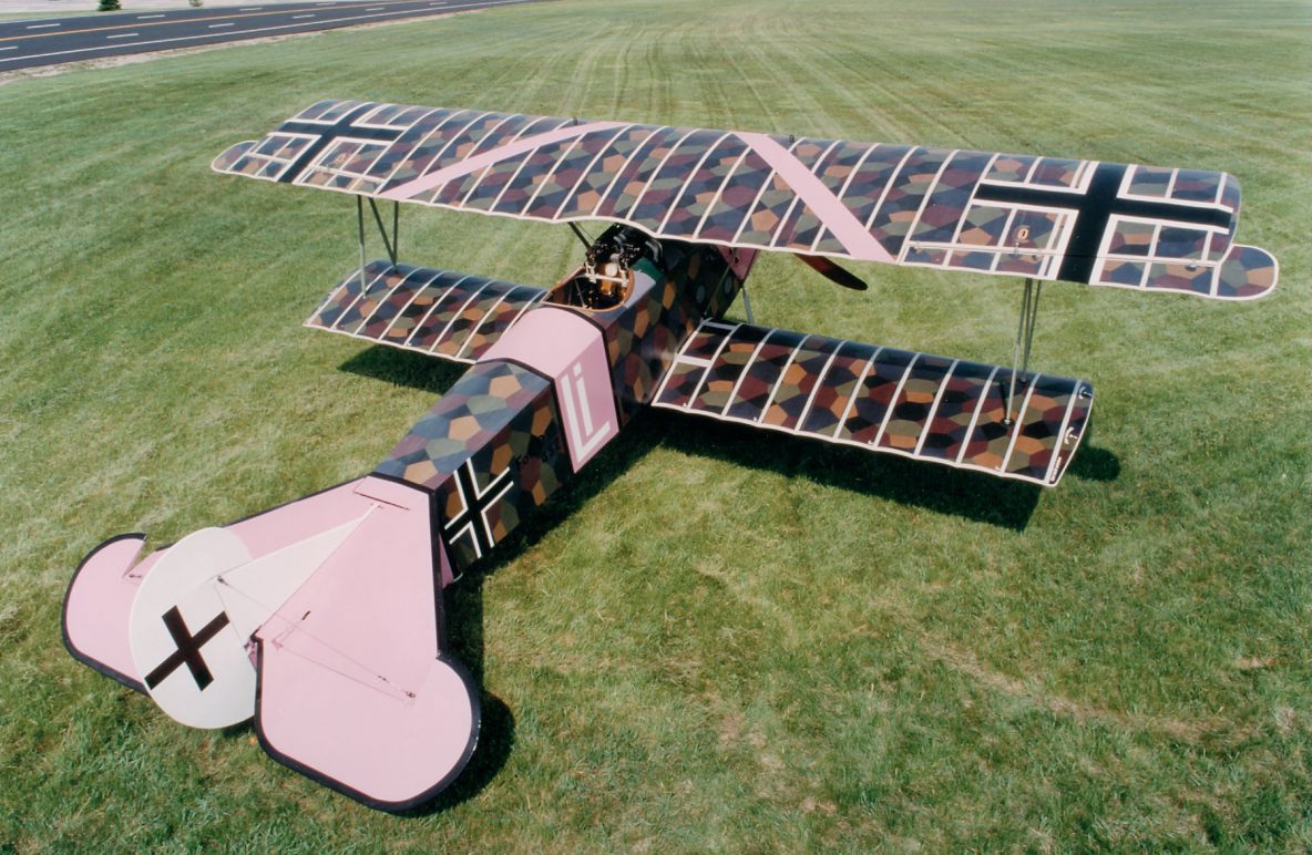
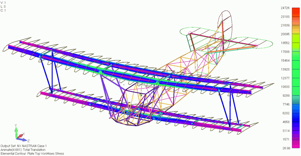

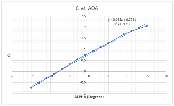
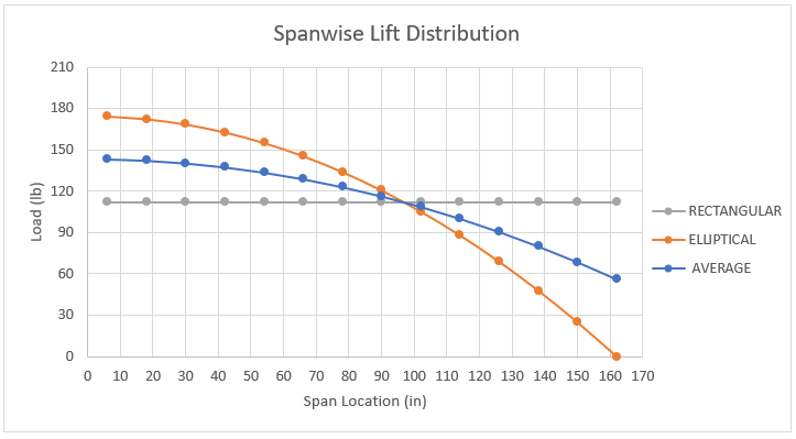
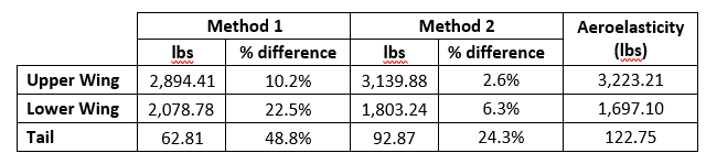
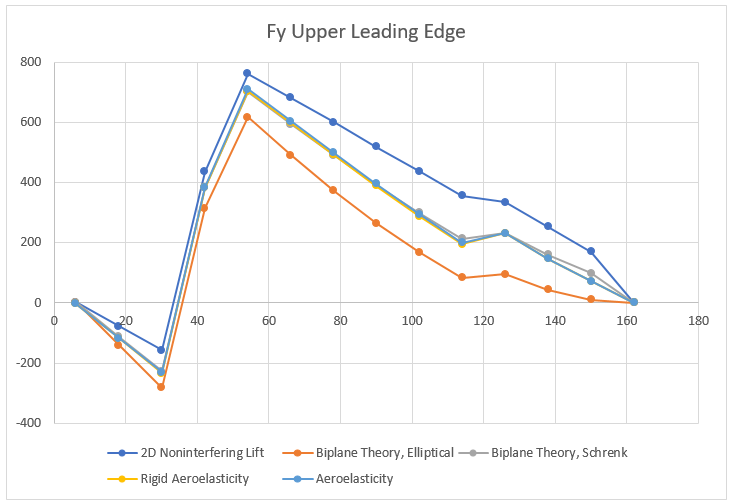
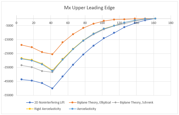
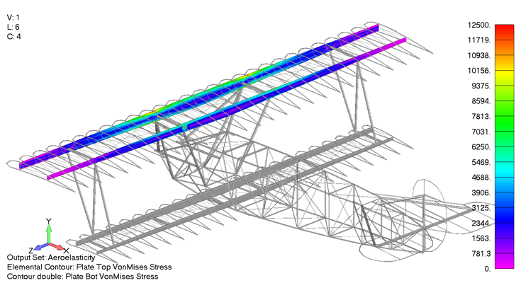
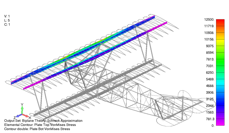
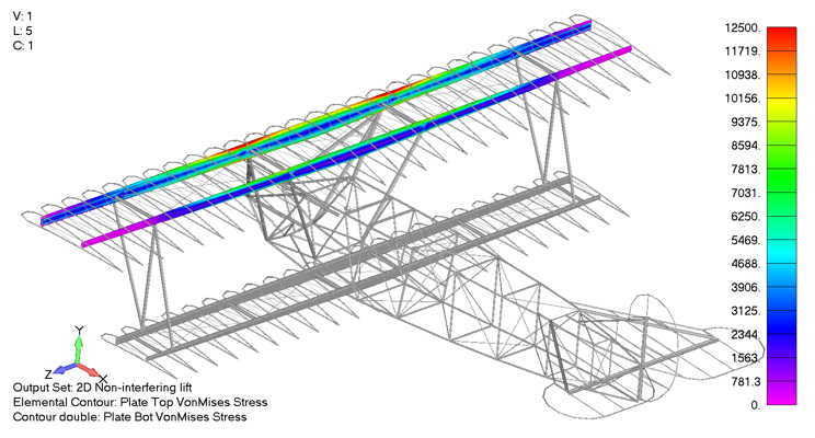
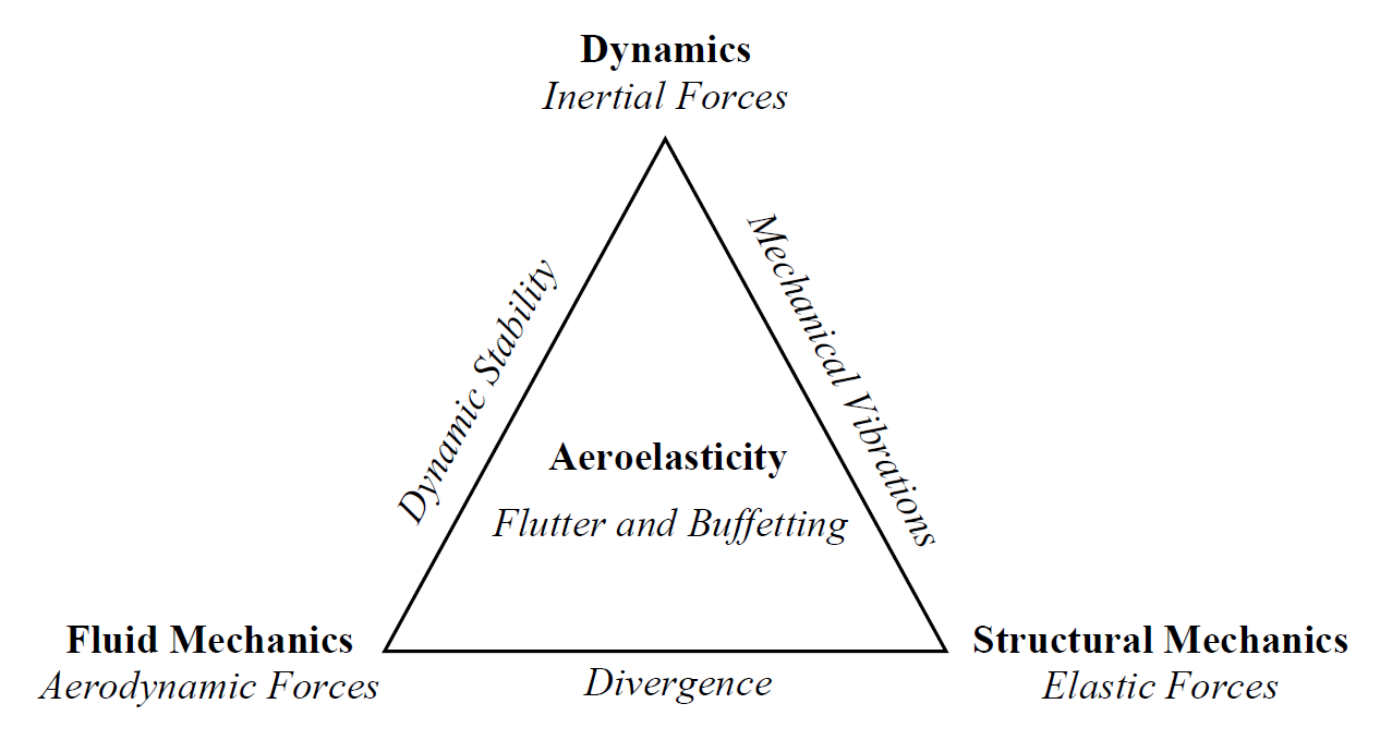


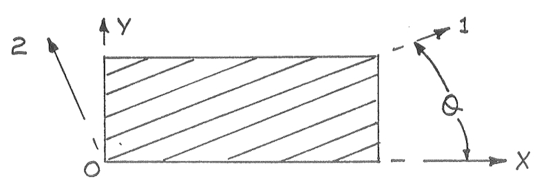
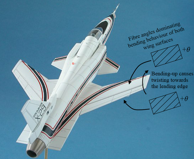

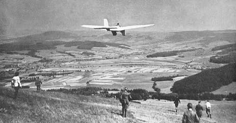

.jpg)
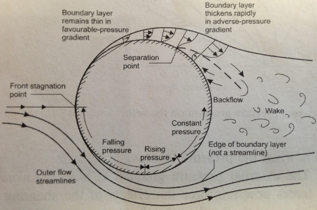


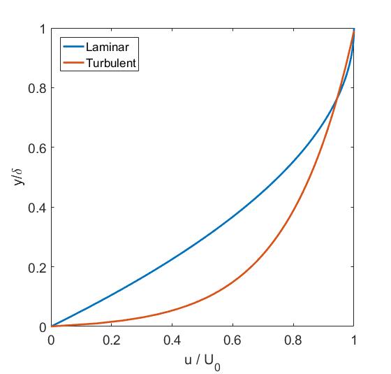
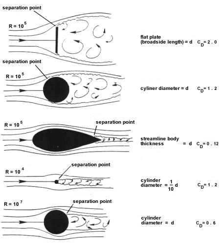
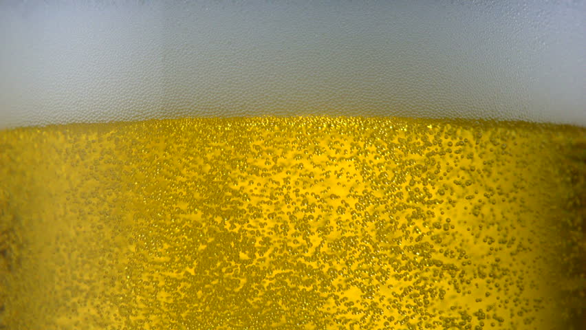


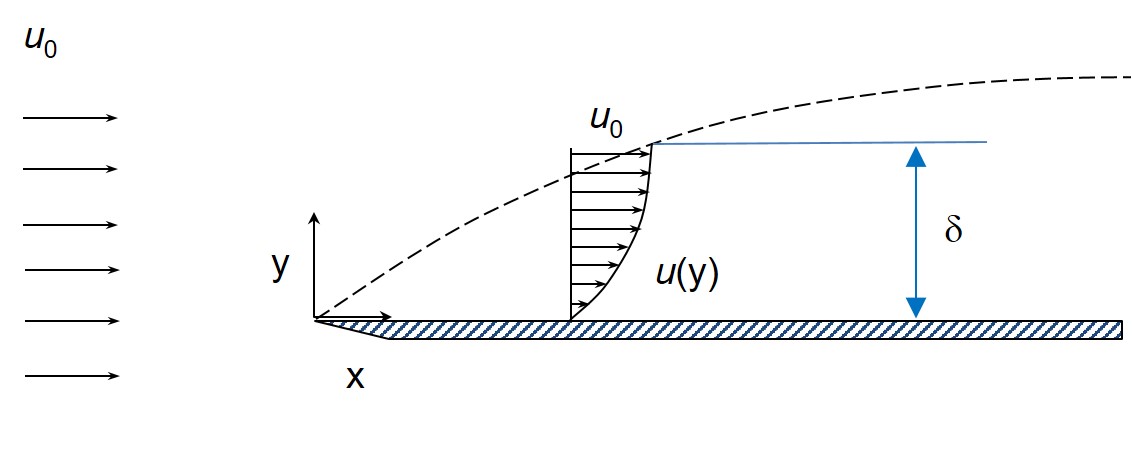
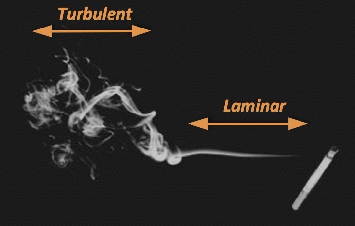

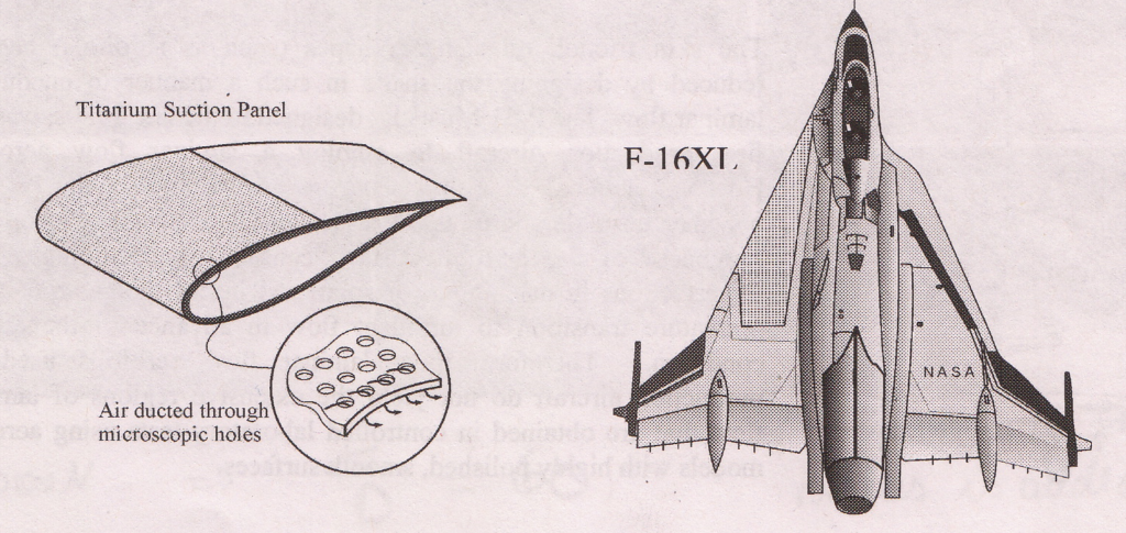

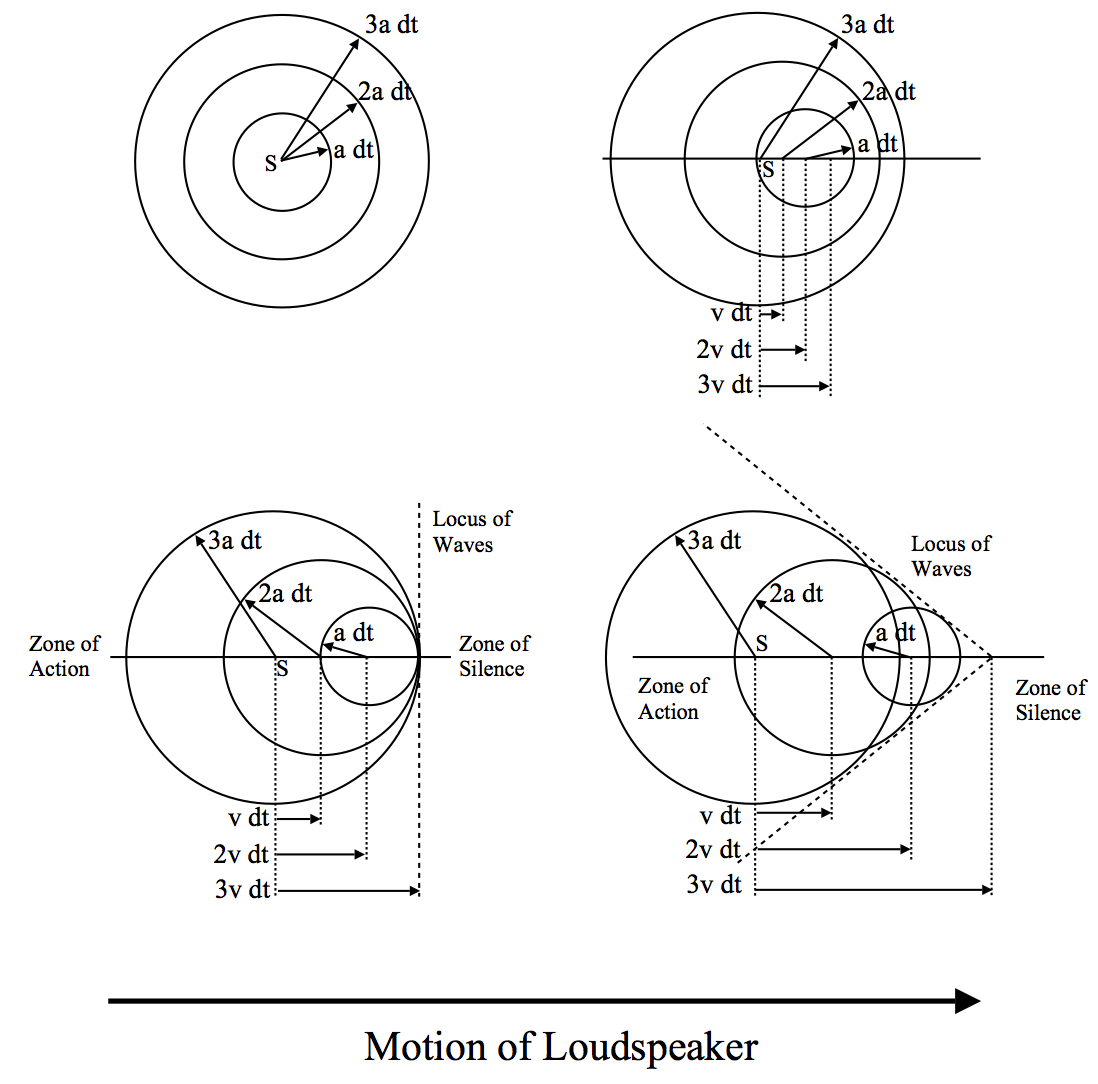

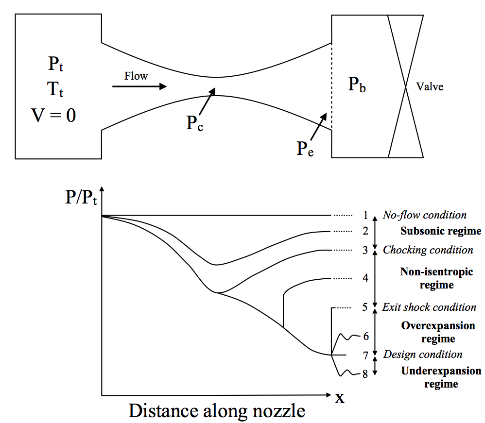

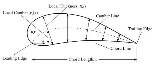
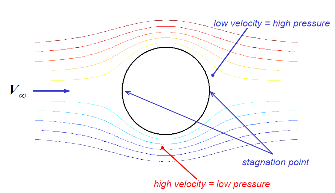
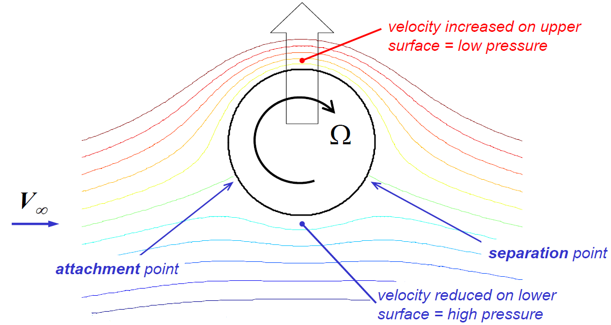
![Flow along a straight streamline [2]](https://rgroh.com/wp-content/uploads/2015/10/Untitled.jpg)
![Flow along a curved streamline [2]](https://rgroh.com/wp-content/uploads/2015/10/Untitled1.jpg)
![Flow around a curved airfoil [2]](https://rgroh.com/wp-content/uploads/2015/10/Untitled2.jpg)